Chapitre 5 Unmeasured confounder

When dealing with an unmeasured confounder, two different scenarios can arise. First the unmeasured confounder can solely act as a confounder without modifying the effect of the exposure on the disease (i.e., no effect measure modification; EMM). In the figure below, the schema on the left illustrate this first scenario. In other situations, the confounder is confounding the exposure-disease association, but is also an EMM of interest, as illustrated by the schema on the right side of the figure. The Bayesian model that we will use to deal with an unmeasured confounder will vary as function of the situation.

Figure. DAG illustrating two types of confounding.

5.1 Unmeasured confounder - no EMM

5.1.1 Lash’s method

When we are simply dealing with an unmeasured confounder that is not expected to be an EMM, an easy option is to run a conventional logistic model using a Bayesian framework, and to simply apply the adjustment described by Lash et al. (2009).¹ within the estimation process.

With:
- $OR\left(biased\right)$ being the biased OR that could be computed using a conventional logistic model;
- $OR\left(ud\right)$ being the hypothesized OR between confounder and disease;
- $PU\left(exp\right)$ being the hypothesized prevalence of the confounder in the exposed;
- $PU\left(unexp\right)$ being the hypothesized prevalence of the confounder in the unexposed.

Then, we can compute an adjusted OR ($OR\left(adj\right)$) describing the relation between exposure and disease after adjusting for the unmeasured confounder as:

$OR\left(adj\right)=OR\left(biased\right)\ast \frac{OR\left(ud\right)\ast PU\left(unexp\right)+1-PU\left(unexp\right)}{OR\left(ud\right)\ast PU\left(exp\right)+1-PU\left(exp\right)}$

We could thus, simply:
1. Provides prior distributions for the intercept, the coefficient of interest, but also for the $OR\left(ud\right)$, $PU\left(exp\right)$, and $PU\left(unexp\right)$. Actually, for $OR\left(ud\right)$, it will be easier to provide a prior for the log of $OR\left(ud\right)$, due to the asymmetry of the OR. NOTE THAT: instead of providing prior distributions for log of $OR\left(ud\right)$, $PU\left(exp\right)$, and $PU\left(unexp\right)$, you could also specify an exact value for these (e.g., PU(exp) = 0.30). The adjustment would then be deterministic, rather than stochastic, for the biased parameters;
2. Develop a conventional logistic Bayesian model;
3. Include the above equation to compute the $OR\left(adj\right)$.

If we use uniform vague distributions for the intercept and the coefficient of interest:

options(scipen=999) # To avoid use of scientific notation by R

mu_int <- 0.0         #mu for the intercept    
inv_var_int <- 0.0001 #Inverse variance for the intercept
mu_betaquest <- 0.0   #mu for the coefficient
inv_var_betaquest <- 0.0001 #Inverse variance for the coefficient

We could use a normal distribution for the log of $OR\left(ud\right)$:

options(scipen=999) 

mu_log_OR_ud <- 1.6         #Mean association (on log odds scale) between confounder and disease (corresponding to an OR of 4.95)   
inv_var_log_OR_ud <- 5      #Inverse variance for the association (on log odds scale) between confounder and disease (corresponding to a variance of 0.2)

We could use beta distributions for $PU\left(exp\right)$ and $PU\left(unexp\right)$, since these are probabilities (i.e., we would like to bound them between 0.0 and 1.0). Here, using the epi.betabuster() function from the epiR library could help. For instance, if we believe that mode for $PU\left(exp\right)$ is 0.60 and that we are 95% certain that it is above 0.50, we could find a corresponding beta distribution for $PU\left(exp\right)$ as follow:

library(epiR) 
rval1 <- epi.betabuster(mode=0.60, conf=0.95, greaterthan=T, x=0.50)  # I create a new object named rval1

rval1$shape1                #View the a shape parameter 

## [1] 42.009

rval1$shape2                ##View the b shape parameter   

## [1] 28.33933

#plot the prior distribution
curve(dbeta(x, shape1=rval1$shape1, shape2=rval1$shape2), from=0, to=1, 
      main="Prior for PU(exp)", xlab = "Proportion", ylab = "Density")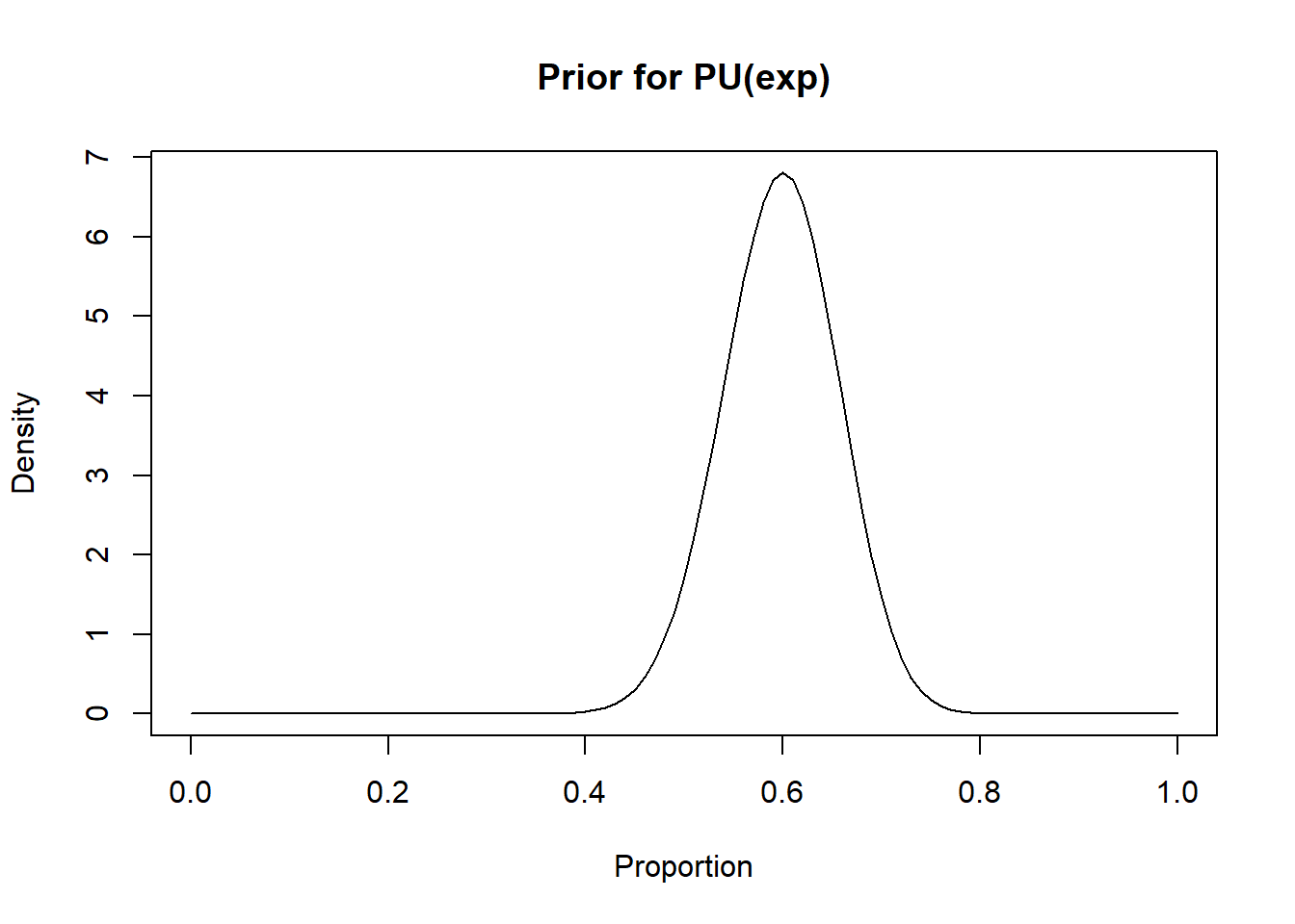

If we believe that mode for $PU\left(unexp\right)$ is 0.20 and that we are 95% certain that it is below 0.30, we could find a corresponding beta distribution for $PU\left(exp\right)$ as follow:

library(epiR) 
rval2 <- epi.betabuster(mode=0.20, conf=0.95, greaterthan=F, x=0.30)  

rval2$shape1                #View the a shape parameter 

## [1] 12.821

rval2$shape2                ##View the b shape parameter   

## [1] 48.284

#plot the prior distribution
curve(dbeta(x, shape1=rval2$shape1, shape2=rval2$shape2), from=0, to=1, 
      main="Prior for PU(unexp)", xlab = "Proportion", ylab = "Density")

With these priors being determined, the following code would create the text file for the model:

# Specify the model:
model_unm_conf_lash <- paste0("model{

#===    LIKELIHOOD  ===#
            for( i in 1 : ",num_obs," ) {
                            test[i] ~ dbern(p[i])
                            logit(p[i]) <- int + betaquest*quest[i]  
            }

#===  EXTRA CALCULATION TO GET OR_biased and OR_adj ===#
            OR_biased <- exp(betaquest)
            OR_adj <- OR_biased*( (OR_ud*PU_unexp+(1-PU_unexp))/(OR_ud*PU_exp+(1-PU_exp)))
            
#===    PRIORS  ===#        
            int ~ dnorm(",mu_int,", ",inv_var_int,")                        #FLAT PRIOR
            betaquest ~ dnorm(",mu_betaquest,", ",inv_var_betaquest,")  #FLAT PRIOR
            
            log_OR_ud ~ dnorm(", mu_log_OR_ud,"," , inv_var_log_OR_ud,")   #PRIOR FOR log_OR_ud     
            OR_ud <- exp(log_OR_ud)                                        #LINK OR_ud TO THE LOG_OR_UD
            
            PU_exp ~ dbeta(", rval1$shape1,",", rval1$shape2, ")               #PRIOR FOR PREVALENCE OF THE CONFOUNDER IN THE EXPOSED INDIVIDUALS 
            PU_unexp ~ dbeta(", rval2$shape1,",", rval2$shape2, ")           #PRIOR FOR PREVALENCE OF THE CONFOUNDER IN THE UNEXPOSED INDIVIDUALS   

        }")

#write to temporary text file
write.table(model_unm_conf_lash, file="model_unm_conf_lash.txt", quote=FALSE, sep="", row.names=FALSE,
 col.names=FALSE)

This code would create the following .txt file:

Note that we could provide initial values for all the unknown parameters. So, not just int and betaquest, but also log_OR_ud, PU_exp, and PU_unexp. For instance:

inits <- list(
  list(int=0.0, betaquest=0.0, log_OR_ud=0, PU_exp=0.20, PU_unexp=0.20),            
  list(int=1.0, betaquest=1.0, log_OR_ud=1.0, PU_exp=0.30, PU_unexp=0.30),
  list(int=-1.0, betaquest=-1.0, log_OR_ud=-1.0, PU_exp=0.10, PU_unexp=0.10)
)

When running the Bayesian analysis, you will have to indicate the parameters that you want to monitor:

library(R2OpenBUGS)
#Set number of iterations
niterations <- 5000
#Run the Bayesian model
bug.out.vague <- bugs(data=cyst, 
                inits=inits, 
                parameters.to.save=c("int", "betaquest", "OR_biased", "OR_adj"),       #I CHOSE TO MONITOR int, betaquest, OR_biased, AND OR_adj  
                n.iter=niterations, 
                n.burnin=0, 
                n.thin=1,
                n.chains=3, 
                model.file="model_unm_conf_lash.txt", 
                debug=FALSE,
                DIC=FALSE)

5.1.2 McCandless’ method

McCandless et al. (2007).² also proposed methods for dealing with an unmeasured confounder when no EMM is present. The advantage of their proposed method is that it can be extended to a scenario where a confounder is also an EMM. In their approach, the unmeasured confounder (UC) is considered as a latent variable. A latent variable is a variable that can not be measured (i.e., it is not in the data set), but that will be included in the model. In that case, it will be included in the model as followed:

$Disease\sim dbern\left(P\right)$
$logit\left(P\right)={\beta }_0+{\beta }_1\ast exposure+{\beta }_2\ast UC$

Of course, since the latent variable UC is not in the data set, we will need to link this latent variable to other parameters. First, we will explicitly link the value (0 or 1) of the unmeasured confounder to the status of the exposure as follow:

$UC\sim dbern\left(Pu\right)$
$logit\left(Pu\right)={\gamma }_0+{\gamma }_1\ast exposure$

So the value of the unmeasured confounder can be 0 or 1, and it has a probability $Pu$ of being 1. This latter probability depends on the exposure status. It makes sense since a confounder has to be associated with the disease of interest, but also with the exposure.

Then, we will make use of the following concepts:
- The hypothesized OR representing the association between the unmeasured confounder and the disease ($OR\left(ud\right)$) can be computed as the exponent of the ${\beta }_2$ coefficient in the first equation ($OR\left(ud\right)=exp\left({\beta }_2\right)$);
- The prevalence of the unmeasured confounder among exposed ($PU\left(exp\right)$) can be estimated using the second equation, through the invert logit function: $PU\left(exp\right)=1/(1+exp(-1\ast ({\gamma }_0+{\gamma }_1)\left)\right)$;
- Similarly, the prevalence of the unmeasured confounder among unexposed: $PU\left(unexp\right)$) can also be estimated ($PU\left(unexp\right)=1/(1+exp(-1\ast \left({\gamma }_0\right)\left)\right)$;

For modelling purposes, it may be more convenient to isolate ${\gamma }_0$ and ${\gamma }_1$ in the latter two equations as follow:

${\gamma }_1=-log\left(1/PU\right(exp)-1)-{\gamma }_0$
${\gamma }_0=-log\left(1/PU\right(unexp)-1)$

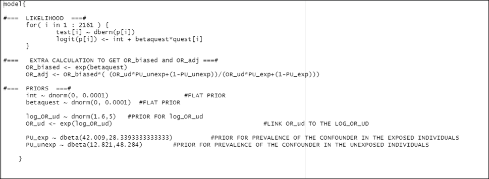
With that, we can create a text file with our model where we will use the exact same unknown parameters as the lash’s method (a coefficient for the intercept ${\beta }_0$, a coefficient ${\beta }_1$ representing the adjusted effect of the exposure, $OR\left(ud\right)$, $PU\left(exp\right)$, and $PU\left(unexp\right)$). Finally, using the coefficient ${\beta }_1$ representing the adjusted effect of the exposure, we will be able to compute the adjusted OR ($OR\left(adj\right)$). Here is how we could create this model. The resulting .txt file is illustrated below.

# Specify the model:
model_unm_conf_McCandless <- paste0("model{

#===    LIKELIHOOD  ===#
            for( i in 1 : ",num_obs," ) {
                            test[i] ~ dbern(p[i])
                            logit(p[i]) <- int + betaquest*quest[i] + betaUC*UC[i]      #UC IS AN UNMEASURED CONFOUNDER (LATENT)
                            
                            UC[i] ~ dbern(Pu[i])           #THE VALUE OF UC HAS PROBABILITY Pu OF BEING 1
                            logit(Pu[i]) <- gamma + gammaquest*quest[i]      #Pu VARIES AS FUNCTION OF THE EXPOSURE STATUS
            }
            
            gamma <- log(1/PU_unexp - 1)*-1             #LINK BETWEEN gamma and PU_unexp
            gammaquest <-  (log(1/PU_exp - 1)*-1)-gamma        #LINK BETWEEN gammaquest AND PU_exp


#===    PRIORS  ===#        
            int ~ dnorm(",mu_int,", ",inv_var_int,")                        #FLAT PRIOR
            betaquest ~ dnorm(",mu_betaquest,", ",inv_var_betaquest,")  #FLAT PRIOR
            
            betaUC ~ dnorm(", mu_log_OR_ud,"," , inv_var_log_OR_ud,")   #PRIOR FOR betaUC WHICH IS SIMPLY OR_ud, BUT ON THE LOG SCALE       
            
            PU_exp ~ dbeta(", rval1$shape1,",", rval1$shape2, ")               #PRIOR FOR PREVALENCE OF THE CONFOUNDER IN THE EXPOSED INDIVIDUALS 
            PU_unexp ~ dbeta(", rval2$shape1,",", rval2$shape2, ")           #PRIOR FOR PREVALENCE OF THE CONFOUNDER IN THE UNEXPOSED INDIVIDUALS   


#===   EXTRA CALCULATION TO GET OR(adj) ===#
            ORquest<-exp(betaquest)
        }")

#write to temporary text file
write.table(model_unm_conf_McCandless, file="model_unm_conf_McCandless.txt", quote=FALSE, sep="", row.names=FALSE,
 col.names=FALSE)

Figure. Model unmeasured confounder (McCandless’ adjustment).

NOTE: McCandless model takes a lot more time to run than the ones where we simply apply Lash’s adjustment. Don’t be surprise if OpenBUGS takes a long time to spit out the results. Moreover, by experience, I see more problems (mainly a high autocorrelation of the Markov Chains) with the McCandless model (vs. the Lash-derived model). So inspect your Markov chains carefully. You may have to run the chains for more iterations to get a sufficient effective sample size. You may also have to use informative priors for all your parameters.

---

1. T. L. Lash, M. P. Fox and A. K. Fink. 2009. Applying quantitative bias analysis to epidemiologic data.↩︎

2. L. C. McCandless, P. Gustafson, and A. Levy. 2007. Bayesian sensitivity analysis for unmeasured confounding in observational studies.↩︎