Chapitre 11 Exposure misclassification
Similar to outcome misclassification, when a binary exposure is subject to error, this can introduce a misclassification bias. Again, the misclassification bias will be described as non-differential, when exposure misclassification is not associated with the outcome or other covariates. It will be described as differential, when misclassification of the exposure is associated with the outcome or with other covariates. Both cases can be handle with a bias analysis.
11.1 Non-differential
Gustafson et al. (2003)4 has proposed a latent class model to handle non-differential misclassification of a binary exposure. In his model, he proposed to model the effect of the true unknown exposure status (a latent class variable) of an individual i, \(Expo(true)_i\), on the probability of disease of this individual, (\(P_i\)), using a logistic regression model. This would be the “response” part of his model.
Response part:
\(Yobserved \sim dbern(P_i)\)
\(logit(P_i) = β_0 + β_1*Expo(true)_i\)
Then, he proposed to link the unknown true exposure status of individual i, \(Expo(true)_i\), and, therefore, the unknown true exposure prevalence \(P(expo)\), to the probability of observing the exposure in individual i (\(P(observed.expo)_i\)), using the sensitivity (\(Se\)) and specificity (\(Sp\)) of the test used to measure the exposure and the observed exposure for individual i \(Expo(observed)_i\). This is the “measurement error” part of his model.
Measurement error part:
\(Expo(true)_i \sim dbern(P(expo))\)
\(Expo(observed)_i \sim dbern(P(observed.expo)_i)\)
\(P(observed.expo)_i = Se*Expo(true)_i + (1-Sp)*(1-Expo(true)_i)\)
So, with this model, if the true exposure status is exposed (or exposure=1), then the probability of being observed as exposed is simply the \(Se\) of the test used to measure the exposure (since on the right part of the equation \((1-1)\) will yield a multiplication by zero). On the other hand, if the true exposure status was unexposed (or exposure=0), then the probability of being observed as exposed is \(1-Sp\) (since the left part of the equation is now multiplied by zero).
To run Gustafson’s model for non-differential-misclassification in R, you will have to:
1. Provide prior distributions (or exact values) for the test’s Se and Sp (Beta distributions could be used, since these are probabilities) and a prior distribution for the unknown true exposure prevalence \(P(expo)\), although this latter can be described using a vague distribution;
2. Modify the R script used to generate the model’s .txt file. For instance, the following script would generate such a .txt file:
# Specify the model:
model_exp_non_dif <- paste0("model{
#=== LIKELIHOOD ===#
for( i in 1 : ",num_obs," ) {
#RESPONSE PART
test[i] ~ dbern(P[i])
logit(P[i]) <- int + betaquest*expo_true[i]
#MEASUREMENT ERROR PART
expo_true[i] ~ dbern(Pexpo)
quest[i] ~ dbern(P_obs_expo[i])
P_obs_expo[i] <- Se*expo_true[i] + (1-Sp)*(1-expo_true[i])
}
#=== EXTRA CALCULATION TO GET OR ===#
ORquest <- exp(betaquest)
#=== PRIOR ===#
int ~ dnorm(",mu_int,", ",inv_var_int,") #PRIOR INTERCEPT
betaquest ~ dnorm(",mu_betaquest,", ",inv_var_betaquest,") #PRIOR COEFFICIENT
Pexpo ~ dbeta(1.0, 1.0) #FLAT PRIOR ON PREVALENCE OF TRUE EXPOSURE
Se ~ dbeta(", rval.se$shape1,",",rval.se$shape2, ") #PRIOR FOR SENSITIVITY
Sp ~ dbeta(", rval.sp$shape1,",",rval.sp$shape2, ") #PRIOR FOR SPECIFICITY
}")
#write to temporary text file
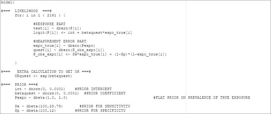
write.table(model_exp_non_dif, file="model_exp_non_dif.txt", quote=FALSE, sep="", row.names=FALSE,
col.names=FALSE)The generated .txt file is illustrated below:
If you prefer to assign fixed values (rather than distributions) for the test’s \(Se\) and \(Sp\), you could modify the last two lines of the R script.
11.2 Differential
Gustafson’s model could be extended to handle differential misclassification of a binary exposure. Similarly to the model for differential outcome misclassification, you will now have to allow the test’s \(Se\) and \(Sp\) to vary according to the value of another variable.
For instance, if we allow the test’s \(Se\) and \(Sp\) to vary according to the value of the outcome, we could rewrite the measurement error part of the model using two equations:
In healthy: \(P(observed.expo)_i = Se_1*Expo(true)_i + (1-Sp_1)*(1-Expo(true)_i)\)
In diseased: \(P(observed.expo)_i = Se_2*Expo(true)_i + (1-Sp_2)*(1-Expo(true)_i)\)
Thus, if an individual is healthy, we will use \(Se_1\) and \(Sp_1\) to link \(Expo(observed)_i\) to \(Expo(true)_i\). In diseased individuals, we will use \(Se_2\) and \(Sp_2\). We will, therefore, have to:
1. Specify exact values or prior distributions for \(Se_1\), \(Sp_1\), \(Se_2\), and \(Sp_2\);
2. Indicate in the model’s .txt file whether, for a given individual, we need to use \(Se_1\) and \(Sp_1\) vs. \(Se_2\) and \(Sp_2\).
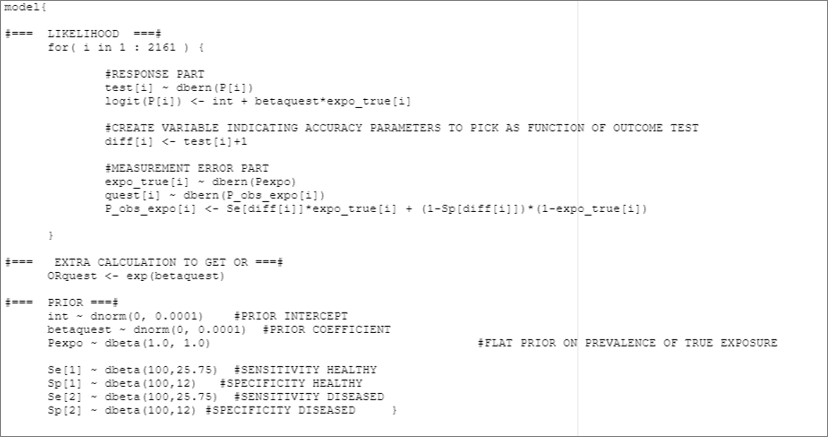
So the complete text file could be generated as follow (after having provided prior distributions or fixed values for \(Se_1\), \(Sp_1\), \(Se_2\), and \(Sp_2\), of course).
# Specify the model:
model_exp_dif <- paste0("model{

#===    LIKELIHOOD  ===#
            for( i in 1 : ",num_obs," ) {

                            #RESPONSE PART
                            test[i] ~ dbern(P[i])
                            logit(P[i]) <- int + betaquest*expo_true[i]

                            #CREATE VARIABLE INDICATING ACCURACY PARAMETERS TO PICK AS FUNCTION OF OUTCOME TEST
                            diff[i] <- test[i]+1

                            #MEASUREMENT ERROR PART
                            expo_true[i] ~ dbern(Pexpo)
                            quest[i] ~ dbern(P_obs_expo[i])
                            P_obs_expo[i] <- Se[diff[i]]*expo_true[i] + (1-Sp[diff[i]])*(1-expo_true[i])

            }

#===   EXTRA CALCULATION TO GET OR ===#
            ORquest <- exp(betaquest)

#===    PRIOR   ===#
            int ~ dnorm(",mu_int,", ",inv_var_int,")        #PRIOR INTERCEPT
            betaquest ~ dnorm(",mu_betaquest,", ",inv_var_betaquest,")  #PRIOR COEFFICIENT
            Pexpo ~ dbeta(1.0, 1.0)                                     #FLAT PRIOR ON PREVALENCE OF TRUE EXPOSURE

            Se[1] ~ dbeta(", rval.se1$shape1,",",rval.se1$shape2, ")    #SENSITIVITY HEALTHY
            Sp[1] ~ dbeta(", rval.sp1$shape1,",",rval.sp1$shape2, ")    #SPECIFICITY HEALTHY
            Se[2] ~ dbeta(", rval.se2$shape1,",",rval.se2$shape2, ")    #SENSITIVITY DISEASED
            Sp[2] ~ dbeta(", rval.sp2$shape1,",",rval.sp2$shape2, ")    #SPECIFICITY DISEASED           }")

#write to temporary text file
write.table(model_exp_dif, file="model_exp_dif.txt", quote=FALSE, sep="", row.names=FALSE,
 col.names=FALSE)
The text file would look as follow: