Chapitre 2 Generating prior distributions
One of the first thing that you will need for any Bayesian analysis is a way to generate and visualize a prior distribution corresponding to some scientific knowledge that you have about an unknown parameter. Generally, you will use information such as the mean and variance or the mode and the 2.5th (or 97.5th) percentile to find a corresponding distribution. You will use various distributions, for instance:
- Normal distribution: defined by a mean (mu) and its standard deviation (SD) or variance (tau). In some software, OpenBUGS for instance, the inverse of the variance (1/tau) is used to specify a given normal distribution. Notation: dNorm(mu, 1/tau)
- Uniform distribution: defined by a minimum (min) and maximum (max). Notation: dUnif(min, max)
- Beta distribution: bounded between 0 and 1, beta distributions are defined by two shape parameters (a) and (b). Notation: dBeta(a, b)
2.1 Normal distribution
The dnorm() function can be used to generate a given Normal distribution and the curve() function can be used to visualize the generated distribution. These functions are already part of R, there is no need to upload a R package.
curve(dnorm(x, mean=2.0, sd=0.5),                                    # I indicate mean and SD of the distribution
      from=-2, to=7,                                                 # I indicate limits for the plot
      main="Normal distribution with mean of 2.0 and SD of 0.5",     #Adding a title
      xlab = "Value", ylab = "Density")                              #Adding titles for axes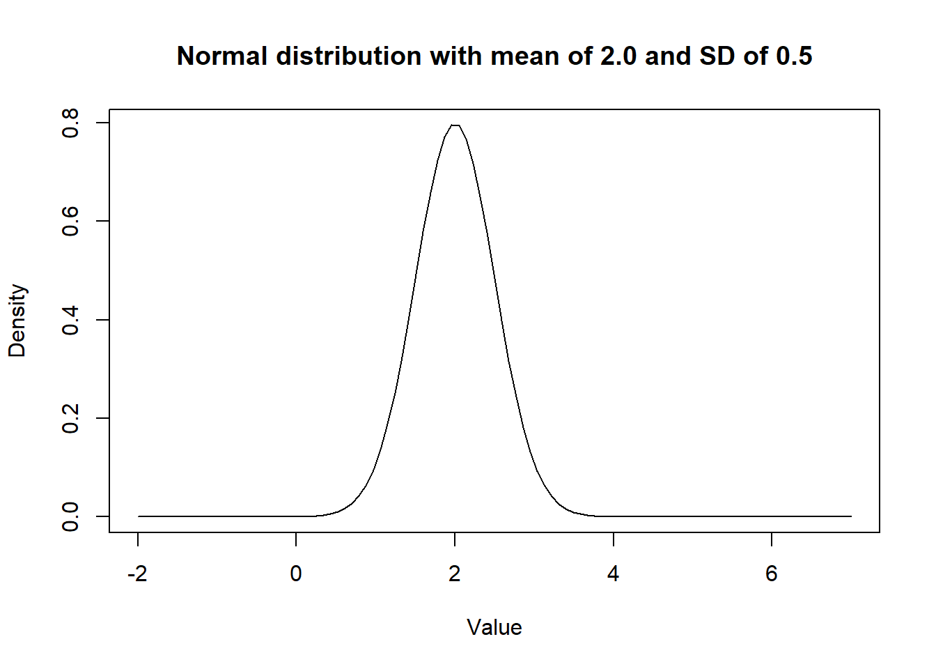
Figure 2.1: Figure. Density curve of a Normal distribution.
Note that a Normal distribution with mean of zero and a very large SD provides very little information. Such distribution would be referred to as a uniform or flat distribution (A.K.A.; a vague distribution).
curve(dnorm(x, mean=0.0, sd=10000000000),
      from=-100, to=100,
      main="A flat Normal distribution",
xlab = "Value", ylab = "Density") 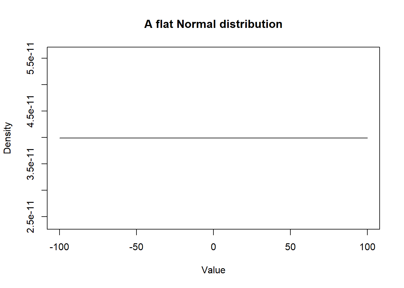
Figure 2.2: Figure. Density curve of a flat Normal distribution.
2.2 Uniform distribution
In the same manner, we could visualize an uniform distribution using the dunif() function. In the following example, we assumed that any values between -5.0 and 5.0 are equally probable.
curve(dunif(x, min=-5.0, max=5.0),
      from=-10, to=10,
      main="Uniform distribution with -5.0 and 5.0 limits",
xlab = "Value", ylab = "Density") 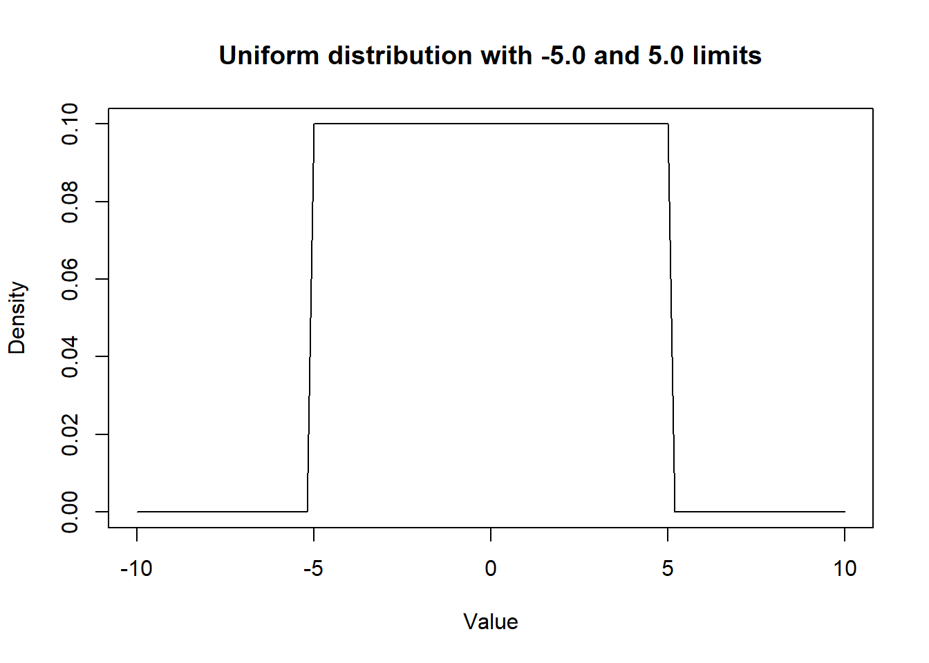
Figure 2.3: Figure. Density curve of an Uniform distribution.
2.3 Beta distribution
Finally, Beta distributions are another type of distributions that will specifically be used for parameters that are proportions (i.e., bounded between 0.0 and 1.0). The epi.betabuster() function from the epiR library can be used to define a given prior distribution based on previous knowledge. When you use the epi.betabuster() function, it creates a new R object containing different elements. Among these, one element will be named shape1 and another shape2. These correspond to the a and b shape parameters of the corresponding Beta distribution.
For instance we may know that the most likely value for the sensitivity of a given test is 0.85 and that we are 95% certain that it is greater than 0.75. With these values, we will be able to find the a and b shape parameters of the corresponding Beta distribution.
library(epiR)

# Sensitivity of a test as Mode=0.85, and we are 95% sure >0.75
rval <- epi.betabuster(mode=0.85, conf=0.95, greaterthan=T, x=0.75)  # I create a new object named rval

rval$shape1                #View the a shape parameter in rval
## [1] 46.348rval$shape2 ##View the b shape parameter in rval ## [1] 9.002588#plot the prior distribution
curve(dbeta(x, shape1=rval$shape1, shape2=rval$shape2), from=0, to=1,
main="Prior for test's sensitivity", xlab = "Proportion", ylab = "Density")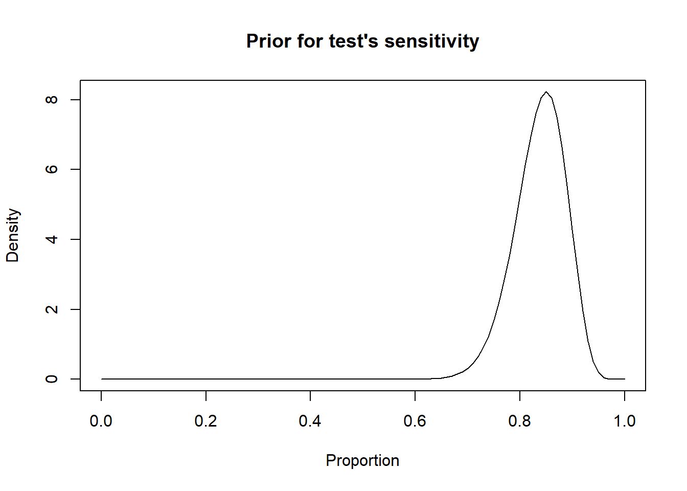
Figure 2.4: Figure. Density curve of a Beta distribution for a test sensitivity.
Note that a dBeta(1.0, 1.0) is a uniform beta distribution.
#plot the prior distribution
curve(dbeta(x, shape1=1.0, shape2=1.0), from=0, to=1,
      main="A Beta(1.0, 1.0) or flat distribution", xlab = "Proportion", ylab = "Density")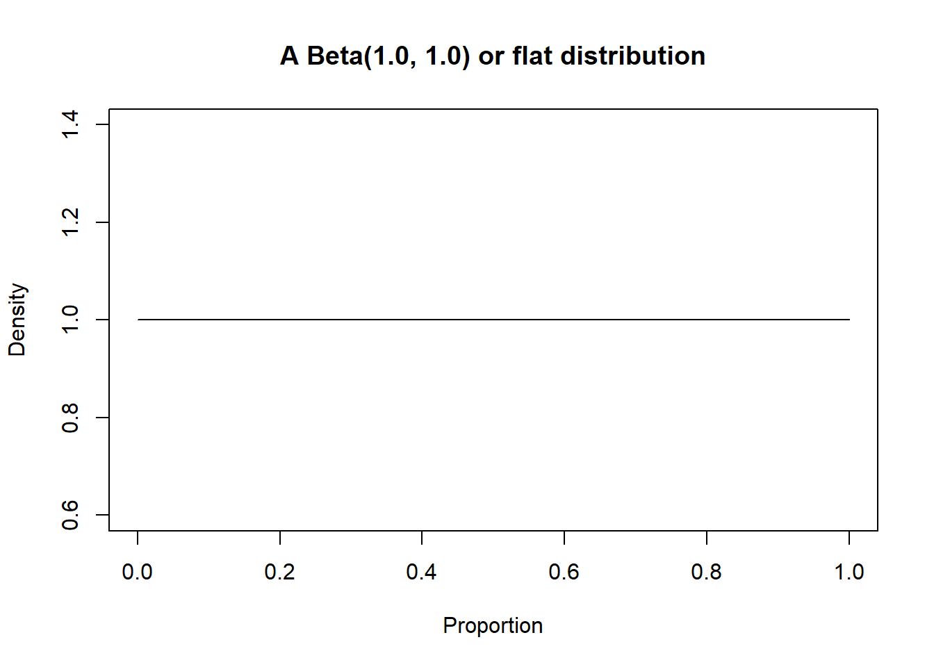
Figure 2.5: Figure. Density curve of a Beta(1.0, 1.0) distribution.