Chapitre 9 Outcome misclassification
When a binary outcome is subject to error, this can introduce a misclassification bias. The misclassification bias will be described as non-differential, when outcome misclassification is not associated with the exposure status, nor with other covariates. It will be described as differential, when misclassification of the health outcome is not equal between exposed and unexposed subjects, or when misclassification is associated with other covariates. Both cases can be handle with a bias analysis.
9.1 Non-differential
McInturff et al. (2004)3 have proposed using a latent class model to handle non-differential outcome misclassification. In their model, they proposed to model the effect of an exposure on the true probability of disease (\(P(true)\)) using a logistic regression model where the disease is a latent class variable (i.e, an unmeasured discrete variable). This is the “response” part of their model. Then, they linked \(P(true)\) to the probability of observing the outcome (\(P(observed)\)), using the test sensitivity (\(Se\)) and specificity (\(Sp\)). This is the “measurement error” part of their model. The model can be written as follow:
\(Yobserved \sim dbern(P(observed))\)
\(P(observed) = Se*P(true) + (1-Sp)*(1-Ptrue)\)
\(logit(P(true)) = β_0 + β_1*quest\)
To run the McInturff’s model for non-differential-misclassification in R, you will have to:
1. Provide prior distributions (or exact values) for the test’s Se and Sp. Beta distributions could be used, since these are probabilities;
2. Modify the R script used to generate the model’s .txt file. For instance, the following script would generate such a .txt file:
# Specify the model:
model_mis_non_dif <- paste0("model{

#===    LIKELIHOOD  ===#
            for( i in 1 : ",num_obs," ) {
                            test[i] ~ dbern(P_obs[i])
                            P_obs[i] <- P_true[i]*Se+(1-P_true[i])*(1-Sp)   #MEASUREMENT ERROR PART
                            logit(P_true[i]) <- int + betaquest*quest[i]  #RESPONSE PART
            }

#===   EXTRA CALCULATION TO GET OR ===#
            ORquest <- exp(betaquest)

#===    PRIOR   ===#
            int ~ dnorm(",mu_int,", ",inv_var_int,")        #FLAT PRIOR
            betaquest ~ dnorm(",mu_betaquest,", ",inv_var_betaquest,")  #FLAT PRIOR

            Se ~ dbeta(", rval.se$shape1,",",rval.se$shape2, ")         #PRIOR FOR SENSITIVITY
            Sp ~ dbeta(", rval.sp$shape1,",",rval.sp$shape2, ")         #PRIOR FOR SPECIFICITY
            }")

#write to temporary text file
write.table(model_mis_non_dif, file="model_mis_non_dif.txt", quote=FALSE, sep="", row.names=FALSE,
 col.names=FALSE)
The generated .txt file is illustrated below:
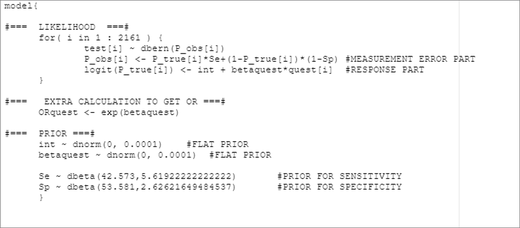
If you prefer to assign fixed values (rather than distributions) for the test’s \(Se\) and \(Sp\), you could modify the last two lines of the R script.
9.2 Differential
The McInturff’s model can be extended to handle differential outcome misclassification. For that, we will have to allow the test’s \(Se\) and \(Sp\) to vary according to the value of another variable. We can make the test accuracy vary as function of the exposure, of another covariate in the model (e.g., a measured confounder), or even another characteristic not even in the model.
For instance, if we allow the test’s \(Se\) and \(Sp\) to vary according to the value of the exposure, we could rewrite the measurement error part of the model using two equations:
In exposed: \(P(observed) = Se_1*P(true) + (1-Sp_1)*(1-Ptrue)\)
In unexposed: \(P(observed) = Se_2*P(true) + (1-Sp_2)*(1-Ptrue)\)
Thus, if exposed, we will use \(Se_1\) and \(Sp_1\) to link (\(P(observed)\)) to (\(P(true)\)). In unexposed individuals, we will use \(Se_2\) and \(Sp_2\). We will, therefore, have to:
1. Specify exact values or prior distributions for \(Se_1\), \(Sp_1\), \(Se_2\), and \(Sp_2\);
2. Indicate in the model’s .txt file whether, for a given individual, we need to use \(Se_1\) and \(Sp_1\) vs. \(Se_2\) and \(Sp_2\).
For the latter, we will simply create a variable that takes value 1 in unexposed (i.e., when quest=0) and value 2 in exposed (i.e., when quest=1). Then, we will incorporate the 1 and the 2 next to our \(Se\) and \(Sp\) in our codes. We can achieve this in OpenBUGS as follow.
This line would assign the value 1 or 2, to unexposed, and exposed, respectively.
diff[i] <- quest[i]+1
We could then modify as follow the measurement error part to assign \(Se_1\) and \(Sp_1\) vs. \(Se_2\) and \(Sp_2\) to a given individual as function of his exposure status:
P_obs[i] <- P_true[i] * Se[diff[i]]+(1-P_true[i]) * (1-Sp[diff[i]])
So the complete text file could be generated as follow (after having provided prior distributions or fixed values for \(Se_1\), \(Sp_1\), \(Se_2\), and \(Sp_2\), of course).
# Specify the model:
model_mis_dif <- paste0("model{
#=== LIKELIHOOD ===#
for( i in 1 : ",num_obs," ) {
diff[i] <- quest[i]+1
test[i] ~ dbern(P_obs[i])
P_obs[i] <- P_true[i]*Se[diff[i]]+(1-P_true[i])*(1-Sp[diff[i]])
logit(P_true[i]) <- int + betaquest*quest[i] #RESPONSE PART
}
#=== EXTRA CALCULATION TO GET OR ===#
ORquest <- exp(betaquest)
#=== PRIOR ===#
int ~ dnorm(",mu_int,", ",inv_var_int,") #FLAT PRIOR
betaquest ~ dnorm(",mu_betaquest,", ",inv_var_betaquest,") #FLAT PRIOR
Se[1] ~ dbeta(", rval.se1$shape1,",",rval.se1$shape2, ") #SENSITIVITY UNEXPOSED
Sp[1] ~ dbeta(", rval.sp1$shape1,",",rval.sp1$shape2, ") #SPECIFICITY UNEXPOSED
Se[2] ~ dbeta(", rval.se2$shape1,",",rval.se2$shape2, ") #SENSITIVITY EXPOSED
Sp[2] ~ dbeta(", rval.sp2$shape1,",",rval.sp2$shape2, ") #SPECIFICITY EXPOSED
}")
#write to temporary text file
write.table(model_mis_dif, file="model_mis_dif.txt", quote=FALSE, sep="", row.names=FALSE,
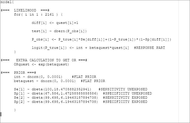
col.names=FALSE)The text file would look as follow:
9.3 Internal validation
If budget allows, one could decide to use a less than perfect test to measure the outcome on all individuals, but also to apply a gold-standard test on a subset of the individuals. The relationship between the imperfect and gold-standard results could be used to generate fixed values or prior distributions for the \(Se\) and \(Sp\) that can then directly be used in McInturff’s latent class model. For instance, we could compile the number of test+, gold standard+, test-, and gold standard- individuals. Using this, we could describe the relation between test+, gold standard+ and test’s \(Se\) as:
\(test+ \sim dbern(Se, goldstandard+)\)
Or, if you prefer, the number of test+ depends on the test’s \(Se\) and the number of true positive. And, for the tests’ \(Sp\):
\(test- \sim dbern(Sp, goldstandard-)\)
Vague priors could be used on the test’s \(Se\) and \(Sp\).