Chapitre 15 Answers to the exercises
15.1 Logistic regression
- Start from the partially completed Question 1.R
Rscript located in Question 1 folder. Use this script as a starting point to compute the crude association between quest and test using a logistic regression model estimated with a Bayesian analysis. Initially, use flat priors for your parameters. Make sure Markov chains’ behaviours are acceptable (i.e., ESS, autocorrelation plots) and that convergence is obtained (i.e., trace plot). How these results compare to those of the unadjusted \(OR\) computed using a frequentist approach (i.e., OR=0.47; 95%CI=0.37, 0.60)?
When we do a quick exam of the associations between quest and test we see that the relationship is a OR of 0.47 (95CI: 0.37, 0.60).
##              Outcome +    Outcome -      Total        Inc risk *        Odds
## Exposed +          137         1142       1279              10.7       0.120
## Exposed -          180          702        882              20.4       0.256
## Total              317         1844       2161              14.7       0.172
##
## Point estimates and 95% CIs:
## -------------------------------------------------------------------
## Inc risk ratio                                 0.52 (0.43, 0.64)
## Odds ratio                                     0.47 (0.37, 0.60)
## Attrib risk in the exposed *                   -9.70 (-12.85, -6.54)
## Attrib fraction in the exposed (%)            -90.53 (-133.87, -55.21)
## Attrib risk in the population *                -5.74 (-8.79, -2.69)
## Attrib fraction in the population (%)         -39.12 (-52.17, -27.19)
## -------------------------------------------------------------------
## Uncorrected chi2 test that OR = 1: chi2(1) = 39.212 Pr>chi2 = <0.001
## Fisher exact test that OR = 1: Pr>chi2 = <0.001
##  Wald confidence limits
##  CI: confidence interval
##  * Outcomes per 100 population units
This OR and 95CI were estimated using a frequentist approach, though. Now, with the Bayesian model…
First, regarding MCMC diagnostics:
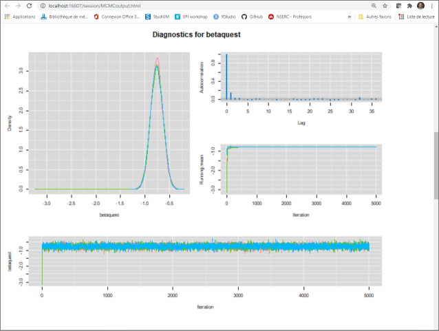
- The trace plot indicate that: 1) all three chains have converged toward the same area; and 2) the burn in period could be relatively short (but we could possibly stick with a burn in of 1,000).
- The plots of the posterior distributions for the intercept, the coefficient of quest, and the OR of quest (which is just a log transformation of the coefficient) are already relatively smooth. So number of iterations, even after applying a burn in period of a 1,000, will probably be sufficient. The EES ranged from 10,433 to 12,066.
- The autocorrelation plots do not indicate any problems with the Markov chains.
Now regarding the results:
##              50%   2.5%  97.5%
## int       -1.362 -1.527 -1.201
## betaquest -0.761 -1.005 -0.519
## ORquest    0.467  0.366  0.595
We see that, when we used a Bayesian estimation with vague prior distributions, the estimated OR (95CI) is 0.47 (0.37, 0.60). Exactly that of the frequentist approach! This was expected, since vague priors were used for all parameters.
We could present the prior and posterior distributions for the coefficient of quest (i.e., the log OR) as shown below.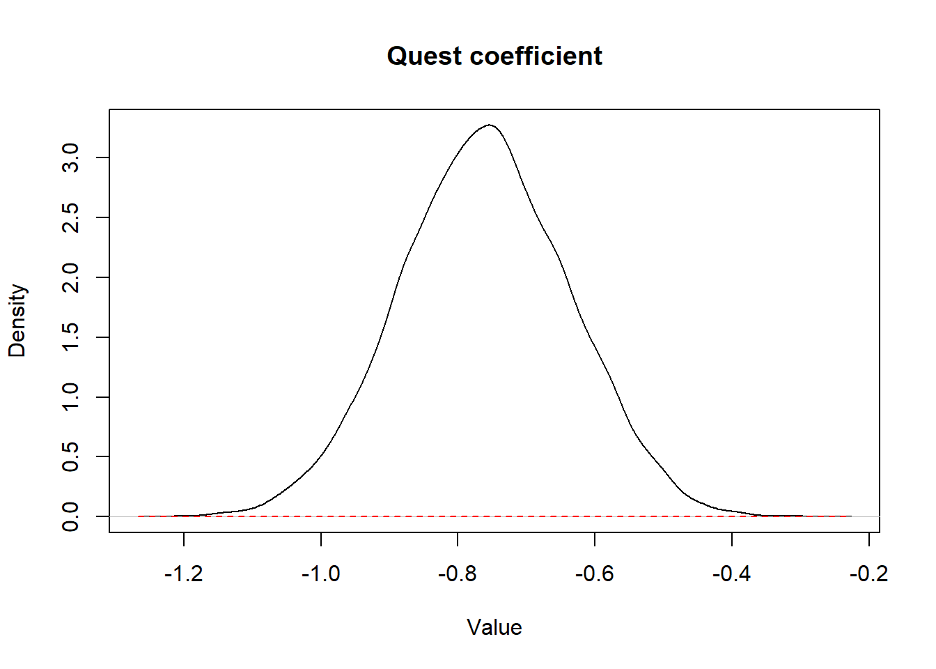
Figure 15.1: Figure. Prior (dashed red) and posterior (full black) distribution for quest coefficient.
- Start from the
Rscript that you completed in Question 1. Run the same Bayesian logistic model, but this time use a prior distribution for quest coefficient that would give equal probability on the log odds scale to values between odds ratio ranging from 0.05 to 20. With such a distribution, you are explicitly saying that, a priori, you do not think the odds ratio could be very extreme, but that all intermediate values are possible. Hint: it is just the prior distributions that need to be modified in two places; 1) when creating yourRobjects and 2) in the model’s text file. How are your results modified?
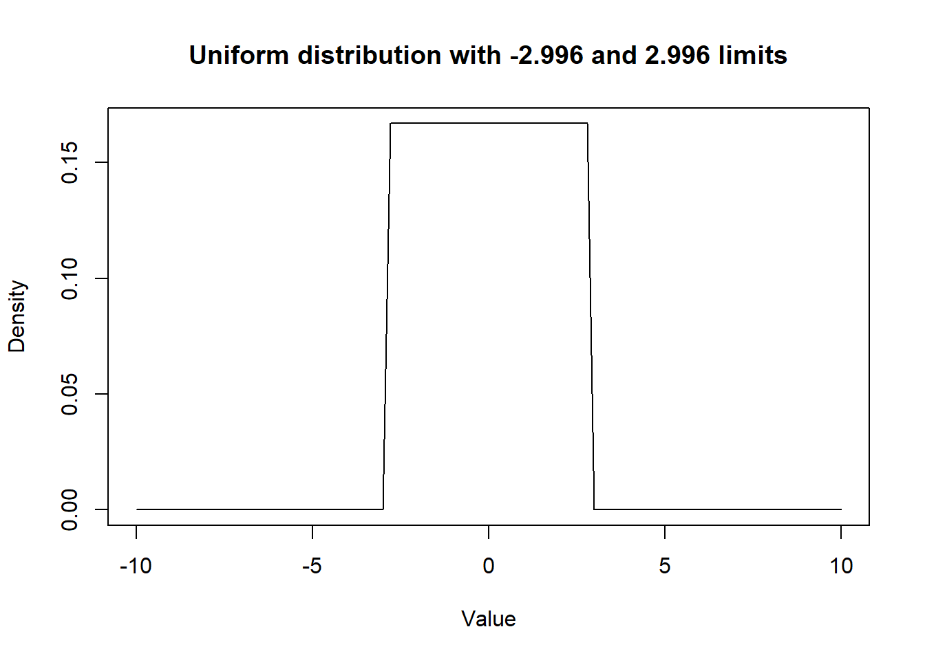
Figure 15.2: Figure. Prior distribution for betaquest.
We can now run the model…
##              50%   2.5%  97.5%
## int       -1.361 -1.527 -1.198
## betaquest -0.761 -1.004 -0.526
## ORquest    0.467  0.366  0.591
Using that prior, after rounding off, the estimated odds ratio is still more or less the same. The OR (95CI) is 0.47 (0.37, 0.59). Actually, there is still very little information in that prior (i.e., we are just excluding OR below 0.05 and above 20 from our prior beliefs). On top of that, we have a relatively large dataset (n=2,161), so the data have a lot of weight compare to the prior distribution.
If we plot the prior and posterior distributions for betaquest we get: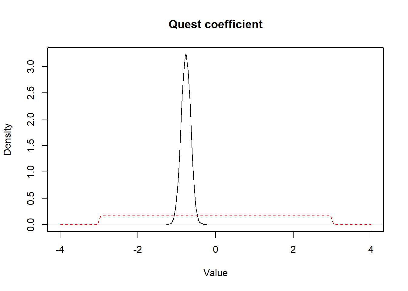
Figure 15.3: Figure. Prior (dashed red) and posterior (full black) distribution for quest coefficient.
- Again, start from the
Rscript that you completed for Question 1 or Question 2. Let go crazy a bit. For instance, you could believe that knowledge does not prevent the disease, but rather will increase odds of cysticercosis. Let say you are very convinced, a priori, that the most probable value for the \(OR\) is 2.0 with relatively little variance in that distribution. Pick a distribution that would represent that prior knowledge. How are your results modified?
I chose to use a dnorm(0.69, 5) as prior for the coefficient for quest. So a normal distribution with mean OR of 2.0 and variance of the log odds would be 0.2 (or SD of 0.45).
This distribution looks like this: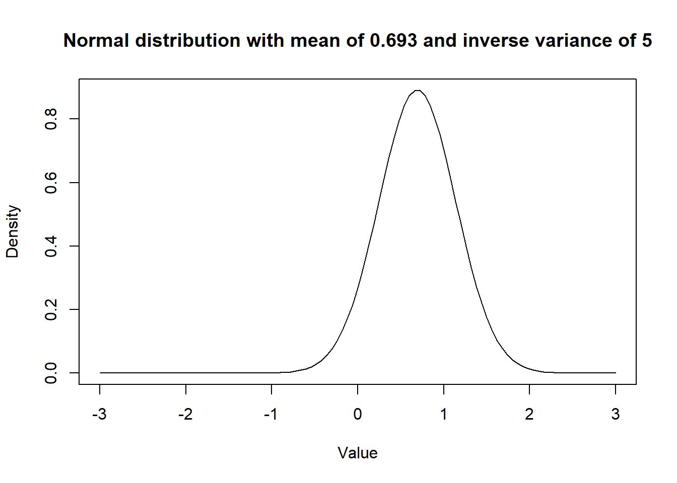
Figure 15.4: Figure. Prior distribution with mean OR of 2.0 and a variance of 0.2.
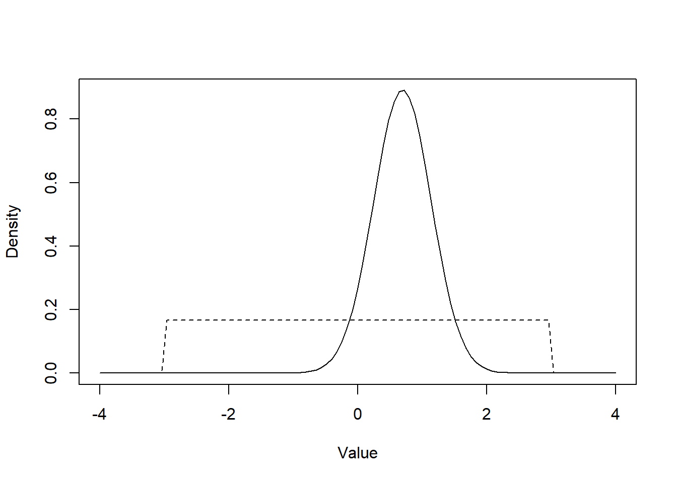
Figure 15.5: Figure. Normal distribution with mean of 0.69 and a variance of 0.20 (full line) vs. unif(-2.996, 2.996) distribution.
When we run this model, we get the following results. (the Markov chains looked appropriate):
##              50%   2.5%  97.5%
## int       -1.410 -1.575 -1.249
## betaquest -0.659 -0.893 -0.426
## ORquest    0.517  0.409  0.653
Using that prior, I get a OR (95CI) of 0.52 (0.41, 0.65). So the estimated odds ratio is now somewhere between our prior knowledge and the frequentist estimate, although still quite close to the frequentist estimate (see next figure). In this case, even with the substantial information contained in our prior distribution, the estimation process is only slightly affected by our prior knowledge. So the dataset size (n=2,161) is still driving most of the estimation process.
We see this quite well, when we plot this very informative prior distribution along with the posterior distribution obtained vs. the posterior distribution of the model where we used a vague prior distribution: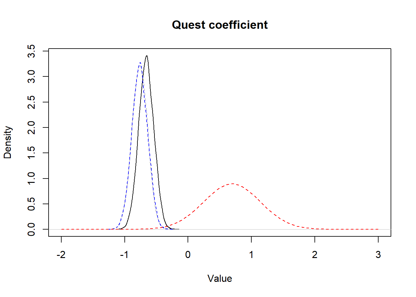
Figure 15.6: Figure. Prior informative distribution with mean of 0.69 and a variance of 0.20 (red dashed) vs. the obtained posterior distribution (full black) and the posterior distribution obtained using vague priors (blue dashed).
- If you have the time… Again, you could modify some of your preceding
Rscripts. To appraise the effect of priors vs. sample size, work on similar analyses, but this time use the cyst_bias_study_reduced.csv data set, which only have 60 observations (compared to 2,161 observations for the complete data set). Run a logistic regression model of the effect of quest on test, using vague prior distributions. Then run the same model, but with the prior distributions that you used in Question 3. Is the effect of the informative priors more important now?
If we explore the crude association in this smaller (n=60) data set using a frequentist approach:
##              Outcome +    Outcome -      Total        Inc risk *        Odds
## Exposed +            5           33         38              13.2       0.152
## Exposed -            4           18         22              18.2       0.222
## Total                9           51         60              15.0       0.176
##
## Point estimates and 95% CIs:
## -------------------------------------------------------------------
## Inc risk ratio                                 0.72 (0.22, 2.42)
## Odds ratio                                     0.68 (0.16, 2.86)
## Attrib risk in the exposed *                   -5.02 (-24.40, 14.35)
## Attrib fraction in the exposed (%)            -38.18 (-361.26, 58.60)
## Attrib risk in the population *                -3.18 (-21.66, 15.29)
## Attrib fraction in the population (%)         -21.21 (-137.09, 38.03)
## -------------------------------------------------------------------
## Yates corrected chi2 test that OR = 1: chi2(1) = 0.023 Pr>chi2 = 0.881
## Fisher exact test that OR = 1: Pr>chi2 = 0.712
##  Wald confidence limits
##  CI: confidence interval
##  * Outcomes per 100 population units
We observed a frequentist OR (95CI) of 0.68 (0.16, 2.9).
If we ran a Bayesian model with vague priors (the Markov chains looked OK), we get:
##              50%   2.5%  97.5%
## int       -1.583 -2.839 -0.554
## betaquest -0.349 -1.882  1.120
## ORquest    0.705  0.152  3.065
An OR (95CI) of 0.71 (0.15, 3.1), quite close to the frequentist estimates.
Now, with a Bayesian model with informative priors in the form of a dnorm(0.69, 5), (again the Markov chains looked OK), we get:
##              50%   2.5%  97.5%
## int       -2.056 -3.041 -1.220
## betaquest  0.412 -0.339  1.203
## ORquest    1.510  0.713  3.332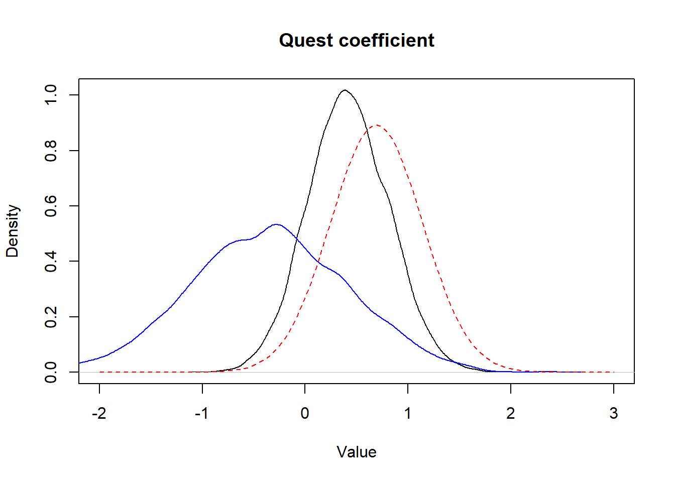
Figure 15.7: Figure. Prior informative distribution with mean of 0.69 and a variance of 0.20 (red dashed) vs. the obtained posterior distribution (full black) and the posterior distribution obtained using vague priors (full blue).
15.2 Unmeasured confounder
- Start from the partially completed Question 1.R
Rscript located in Question 1 folder. Try to adjust the OR obtained from a conventional logistic model using Lash’s method. Use vague priors for the intercept and the coefficient of your logistic model. assume that you are not 100% sure about the values that should be used for your bias parameters, so use distributions for these, rather than exact values. For instance we could assume that:
- Log of the unmeasured confounder-disease OR (\(OR(ud)\)) follows a normal distribution with mean of 1.6 (i.e., a OR of 5.0) and variance of 0.2 (i.e., an inverse variance of 5.0);
- Prevalence of confounder in exposed (\(PU(exp)\)): mode=0.60 and 5th percentile=0.50;
- Prevalence of confounder in unexposed (\(PU(unexp)\)): mode=0.20 and 95th percentile=0.30.
How these results compare to the one obtained with the QBA analyses?
The Markov chains looked OK. Median adjusted OR is 0.26 (virtually unchanged as compared to the QBA analysis), but 95%CI are now 0.16 to 0.39, so slightly larger. This is expected because we are now not only considering uncertainty due to sample size, but also uncertainty in our bias parameters. Below, I plotted the posterior distributions for the adjusted (full black) and biased (red dashed) OR.

Figure. Posterior distributions for the adjusted (full black) and biased (red dashed) OR.
- Start from the
Rscript that you completed in Question 1. To investigate effect of the imprecision in your bias parameters, change the normal distribution for the log of the unmeasured confounder-disease OR. Keep a mean of 1.6, but use a larger variance, for instance 1.0 (i.e., an inverse variance of 1.0). How is your CI affected?
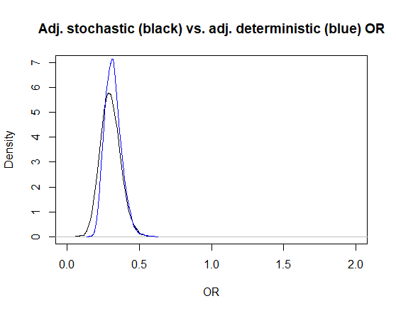
Again, Markov chains are fine. The median adjusted OR (95CI) is now 0.27 (0.14, 0.55). So the median estimate has not changed much, but the 95CI is larger. This is well visible on the following figure where I have plotted the posterior distributions of the biased OR (red dashed), of the adjusted OR assuming a variance of 0.2 of the unmeasured confounder-disease OR (blue) as well as the one assuming a variance of 1.0 (black) of this latter parameter.
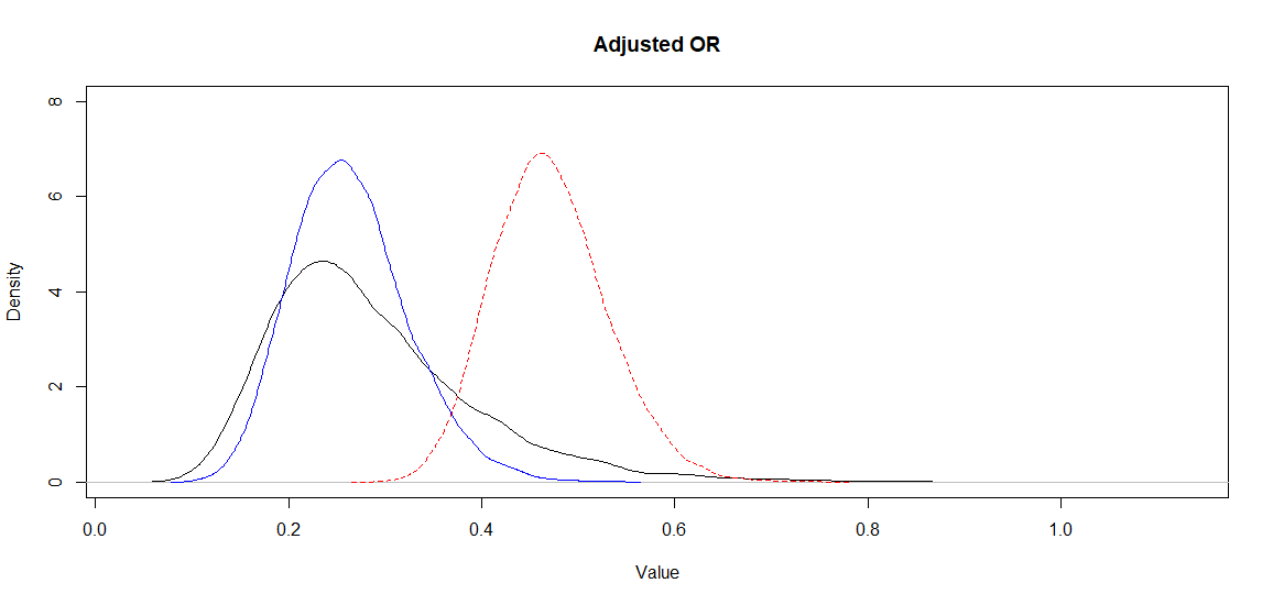
Figure. Posterior distributions for the adjusted (black and blue) and biased (red dashed) OR.
- Start from the partially completed Question 3.R
Rscript located in Question 3 folder. Re-investigate this bias analysis using the alternative model proposed by McCandless. Use the same bias parameters distributions proposed in question 1. Do you get similar results? Note that this later model could easily be expanded to add effect measure modification (i.e., an interaction term between exposure and confounder). Using that expanded model, you could then report effect of exposure by strata of confounder.
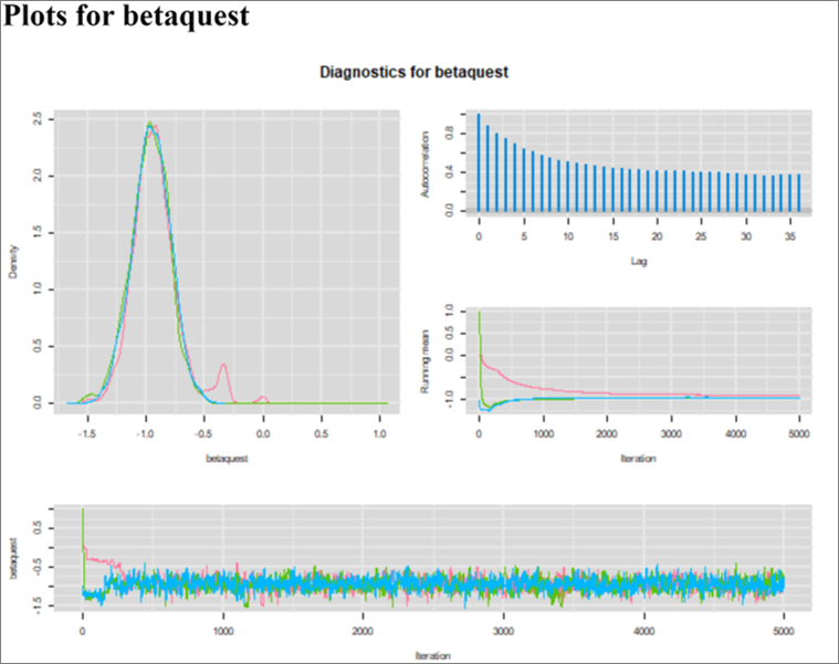
When running this model, there was some issues with the Markov chains. It took almost 800 iterations for convergence, and the autocorrelation of the Markov chains is maintained for iterations that are many steps apart. This is translated in the trace plots, where we can still see the chains cycling up and down slightly (though they are still moving in a relatively very narrow space after 800 iterations). This is also translated in the ESS that is relatively small. This unwanted feature could be overcome by running the chains for a longer number of iterations.
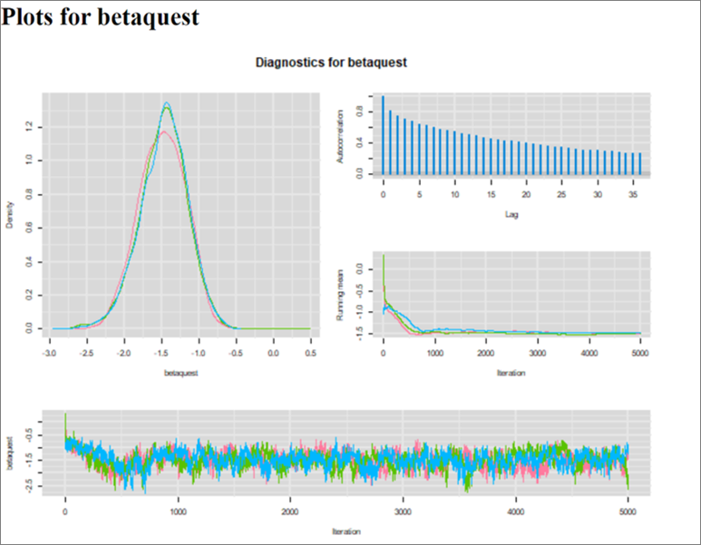
Figure. Diagnostic plots.
If it was for a publication, (vs. our exercise!), we could also investigate whether using informative priors for all unknown parameters would help. By experience, latent class models are more prone to these kind of issues. For now, I ran the chains for 15,000 iterations with a burn in of 1,000. With that the EES was > 1,100 for all parameters.
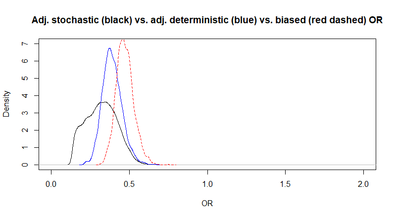
Using McCandless’s method, we obtained a median adjusted OR (95CI) of 0.23 (0.12, 0.38) which is very close to the one obtained with Lash’s adjustment using the same bias parameters (in question 1). To illustrate this, I plotted the posterior distributions for the adjusted OR using McCandless (black) vs. Lash (blue) vs. the biased OR (red dashed)
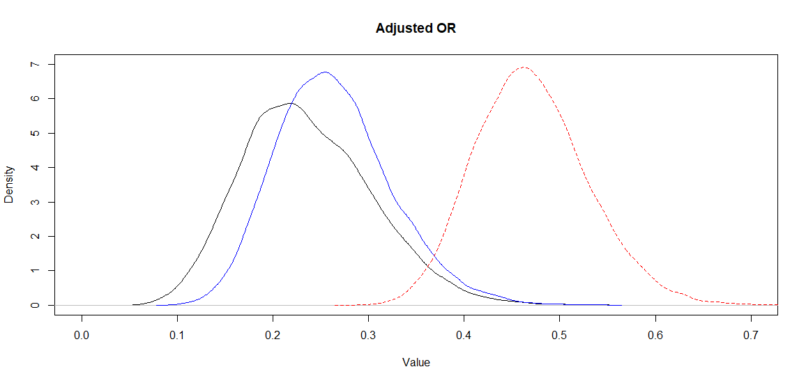
Figure. Posterior distributions for the adjusted (black and blue) and biased (red dashed) OR.
15.3 Selection bias
- Start from the partially completed Question 1.R
Rscript located in Question 1 folder. Try to adjust the OR obtained from a conventional logistic model using the equation provided during the lecture on selection bias. Use vague priors for the intercept and the coefficient of your logistic model. As a first step, for the bias parameters use a deterministic approach (i.e., exact values) rather than prior distributions. How these results compare to that of exercise #5? What is going on?
The adjusted and biased OR are exactly the same: 0.47 (95CI: 0.37, 0.60). There is no bias because \(OR(sel)\) is:
\(OR(sel) = \frac{0.25*0.30}{0.75*0.10} = \frac{0.075}{0.075} = 1\)
Thus, the biased OR has to be multiplied by 1 to obtain the adjusted OR (i.e., with these selection probabilities, there is no selection bias).
- Modify the
Rscript that you have completed for Question 1. Now assume that selection probability among diseased unexposed is also 0.75. For now stick with a deterministic approach (i.e., exact values) rather than prior distributions for bias parameters. Is there a selection bias in that case?
There will very likely be a selection bias in that case, since:
\(OR(sel) = \frac{0.75*0.30}{0.75*0.10} = \frac{0.25}{0.075} = 3.33\)
The adjusted OR was 1.4 (95CI: 1.1, 1.8) while the biased OR was 0.47 (95CI: 0.37, 0.60). Below is a plot of the biased vs. adjusted OR.
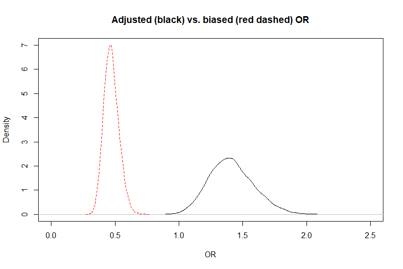
When looking at the figure, it gives the impression that the posterior distribution for the adjusted OR is wider. This should not be the case, since we used a deterministic approach. It is simply an artifact of the scale on which it was measured. If we compare the biased and adjusted association on a log(odds) scale (see below), there is no differences anymore.
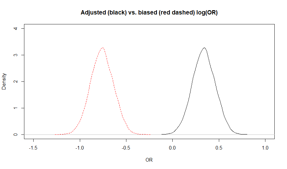
Figure. Posterior distributions for the biased (red dashed) vs. adjusted (black) OR.
- Modify the
Rscript that you have completed for Question 2. Use these same bias parameters, but now propose distributions for these. For instance, you could use the proposed selection probabilities as modes of the distributions and have the 5th or 95th percentiles fixed at -10 or +10 percentage-points from that mode. How do your results differ from that of Question 2?
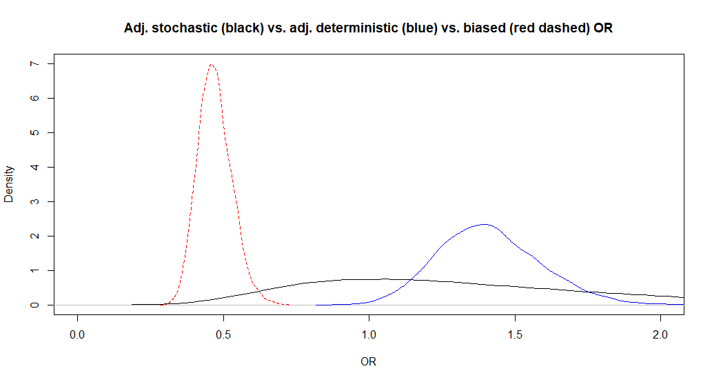
The adjusted OR is now 1.3 (95CI: 0.55, 3.6). So the median adjusted OR is almost unchanged, but the 95CI is larger, as expected. It is because we are now considering uncertainty around the bias parameters in addition to the uncertainty due to the sample size. Below, I have plotted this adjusted OR along with those from Question 2.
- If you have the time, repeat the analyses from Question 3, but with 5th or 95th percentiles at -20 or +20 percentage-points from the modes.
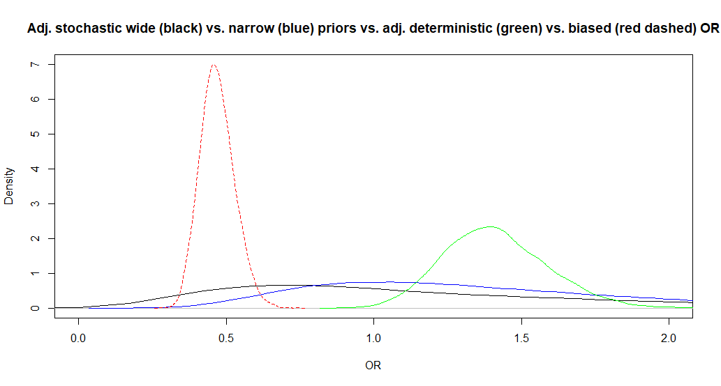
The adjusted OR is now 1.1 (95CI: 0.29, 6.4). So the median adjusted OR is slightly changed and the 95CI is even larger. Below, I have plotted this adjusted OR along with those from Question 2 and 3 for for biased (red dashed), adjusted stochastic with wide (black) vs. narrower (blue) prior distributions for bias parameters, or adjusted deterministic OR (green).
15.4 Outcome misclassification
1. Start from the partially completed Question 1.R R script located in Question 1 folder. Develop a latent class model that would provide an OR adjusted for outcome misclassification. As a first analysis, use point estimates for the Se and the Sp (i.e., use a deterministic approach). Try the value 1.0 for Se and Sp. Thus, you would now have a
model that explicitly admit that Se and Sp of the diagnostic test is perfect. How do these results differ from the conventional logistic model?
As expected, we get an OR (95% CI) of 0.47 (0.37, 0.59) which is the same as the conventional logistic model (which implicitly state that Se and Sp are perfect). However, for the first time we can observe Markov chains that are slightly less than perfect. For instance, we now see a bit of autocorrelation (see Figure below). Nothing dramatic though, these are still very acceptable. The EES ranged from 981 to 1316, depending on the parameter.
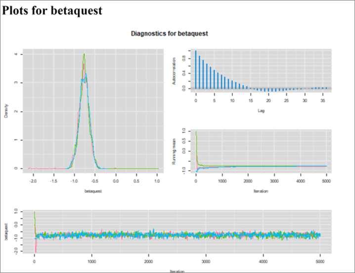
Figure. Diagnostic plots.
Why is it happenning? When using the value 1.0 for the test Se and Sp, the model should be mathematically equivalent to a conventional logistic model (i.e, a model with just a response part). The model is indeed the same, but the Markov chains are not. This is because of the way OpenBUGS interprets the code to automatically construct the chains. OpenBUGS does not realize the redundancies in the code when Se=1 and Sp=1, and therefore comes up with unnecessarily complex chains.
2. Modify the R script that you have completed for Question 1. Stick with the deterministic approach, but now use Se=0.90 and Sp=0.97. Are the results similar to those of exercise #5 from the QBA part of the course?
We get an OR (95CI) of 0.39 (0.28, 0.53). Very similar to what we had using EpisensR. We still have the autocorrelation problem with the Markov chains. Actually, the MC also took more time (approx. 300 iterations) to reach convergence.
3. Modify the R script that you have completed for Question 2. Now use a probabilistic approach where distributions are used to describe your knowledge about Se and Sp of the diagnostic test. For instance, in the literature you may have found that, for the Se, a distribution with mode=0.90 and 5th percentile=0.80 would be realistic. Similarly, the Sp could be described with a distribution with mode=0.97 and 5th percentile=0.90. What is you prediction (a priori) regarding your results? You may have to use informative priors for your unknown parameters. You will possibly have to have a long burn in period and run for many iterations, etc…
If you used vague prior for your unkown parameters, the first thing you will notice is that the Markov chains are awful! I kept the Monte Carlo simulation running for 20,000 iterations and convergence was still not obtained. Actually, when the latent class model is run with distributions for the Se and Sp estimates and vague priors for our intercept and predictor, a single solution cannot be identified anymore. Hence the Markov chains that could not move toward a definite space, representative of the posterior distribution.
For that model to work, you will need to commit yourself and add some prior knowledge regarding your unknown parameters. For this model, I have tried different approaches. In the end, I chose to use a dUnif(-2.0, 2.0) for the intercept, as well as for the coefficient of quest. Thus, my prior beliefs are that:
- the OR would not be smaller than 0.14 or greater than 7.4.
- the prevalence of disease in unexposed is > 0.12 and < 0.88.
These are moderately informative priors, but remember that they will be overridden by our large data set. These priors seemed sufficient for improving our Markov chains. Actually, dUnif(-3.0, 3.0) were also improving the Markov chains a lot and could, perhaps, be more acceptable? They would correspond to OR between 0.05 and 20.0 and to prevalence of disease in unexposed between 0.05 and 0.95.
Moreover, I also ran the Markov chains for 15,000 iterations and applied a burn in period of 5,000. Below are the diagnostic plots with these parameters. The ESS with these parameters ranged from 613 to 696, depending on the parameters. We could run it to generate a larger ESS if it was for publication.
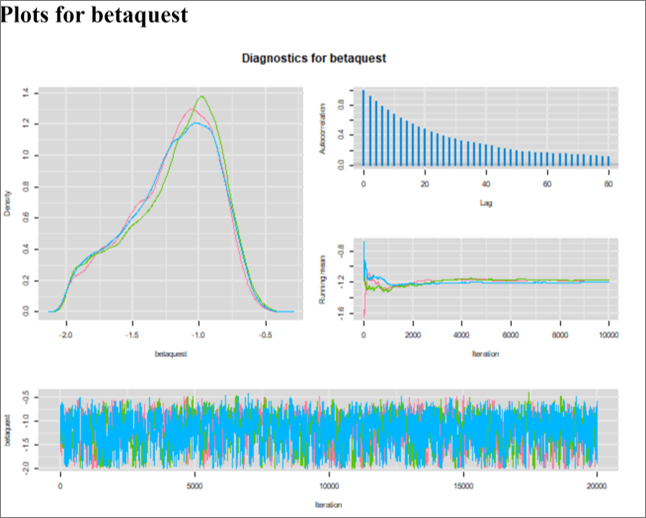
The OR is slightly modified at 0.32 (note that 0.32 and 0.39 is not a huge difference for an OR), but the 95CI is larger at 0.15 to 0.51. Below, I have plotted the unadjusted OR (red dashed), along with the OR adjusted using a deterministic (blue) vs. stochastic (black) approach.
Why was the median OR estimate modified in that case? In most other exercises, when we switched from a deterministic to a probabilistic approach, the 95CI was enlarged, but the OR point estimate was the same…
When a disease is relatively uncommon, a loss of specificity of a few percentage-points may yield a large bias because a large number of healthy individuals will be misclassified as sick. For instance, with 10 truly sick and 100 truly healthy, a 5 percentage-points drop in Se will lead to misclassification of 0.5 individual (from truly sick to diagnosed as healthy). In comparison, with the same drop in Sp we would have 5 truly healthy individuals diagnosed as sick. By specifying a Sp distribution with mode of 0.97, but especially with 5th percentile of 0.90, which allows Sp to be lower than 0.97, we increase the possibility for a larger bias.
4. Start from the partially completed Question 4.R R script located in Question 4 folder. Using the same data, develop a model that would allow for differential outcome misclassification (i.e., different Se and Sp values in exposed and unexposed). First, start with a deterministic approach. For instance, use Se=0.85 and Sp=0.99 in unexposed and Se=0.95 and Sp=0.95 in exposed.
This time the Markov chains are appropriate. I got an OR (95CI) of 0.22 (0.15, 0.32).
5. Modify the R script that you have completed for Question 4. Now use distributions for your bias parameters. Use the previously proposed values as modes for the distributions, and mode minus 5 percentage-points as 5th percentiles. You will probably have to use informative priors for the quest coefficient. You will possibly have to have a long burn in period and run for many iterations, etc…
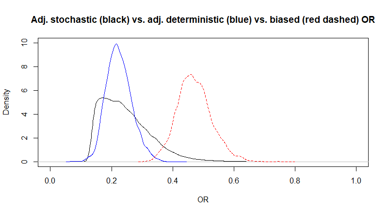
Again, here I used informative priors: dUnif(-2.0, 2.0) for the intercept, as well as for the coefficient of quest. And I had to “fine tune” the MCMC analysis: 15,000 iterations, and a burn in period of 5,000 to get decent ESS. With that, I had a median OR of 0.23 (95CI: 0.14, 0.44). Below I plotted the unadjusted OR (red dashed), along with the OR adjusted for differential misclassification using a deterministic (blue) vs. stochastic (black) approach.
15.5 Exposure misclassification
- Start from the partially completed Question 1.R
Rscript located in Question 1 folder. Using a Bayesian model compute a OR adjusted for exposure misclassification. First use a deterministic approach (using the bias parameters values proposed).
The Markov chains are nice. With this deterministic approach we get an OR (95CI) of 0.31 (0.22, 0.44).
- Modify the
Rscript that you have completed for Question 1. Now use distributions for the bias parameters using values proposed as modes, and mode minus 5 percentage-points for the 5th percentile.
Autocorrelation was present, and, with 5,000 iterations, I had an ESS ranging from 217 (for the intercept) to 419 (for the OR). I increased the number of iterations and then had EES ranging from 547 (for the intercept) to 1002 (for the OR). If it was for publication, we could certainly let it run more to get larger EES.
With the probabilistic approach, I got an OR of 0.30 (95CI: 0.17, 0.45).
Below, I plotted the posterior distributions for the adjusted OR estimated using the deterministic (blue) and stochastic (black) approaches. Note that they are not very different, since we used very narrow distributions with the stochastic approach for the Se and Sp of the test used for measuring the exposure.
- Modify the
Rscript that you have completed for Question 1. We will now explore the potential impact of differential misclassification of quest. Suppose that the Se of the test to measure knowledge about cysticercosis is exactly (deterministic approach) 0.90 among test+ individuals and 0.70 among test- and that the Sp is 0.95 among test+ and 0.85 among test-. Is the misclassification bias larger or smaller than in #1?
With this differential bias, we now have an adjusted OR (95CI) of 0.14 (0.09, 0.21). So the differential exposure misclassification bias was creating a larger bias (from an OR of 0.14 to 0.47) than the non-differential (from an OR of 0.30 to 0.47).
- If you have the time, modify the
Rscript that you have completed for Question 3. Now, include some uncertainty around the estimates provided in Question 3 by adding 5th percentiles located 10 percentage-points from the proposed value (e.g., mode at 0.90, 5th percentile at 0.80). What has changed?
With these parameters, the Markov chains were not converging. I tried with dunif(-2.0, 2.0) priors for the intercept and coefficient (we used them before for another LCM). I also specified a dunif(0.30, 0.70) for prevalence of truly exposed individuals, and ran it for 10,000 iterations. With these parameters, the Markov chains were improved, but the ESS were still small. I am still working on it!
15.6 Multiple biases
- Start from the partially completed Question 1.R
Rscript located in Question 1 folder. Using a Bayesian model compute an OR adjusted for unmeasured confounding, misclassification of exposure, and selection bias. In this case, in which order will you have to organize your biases adjustments? First use a deterministic approach (using the bias parameters values proposed, but ignoring the provided 5th and 95th percentiles or any other measures of spread of the distributions).
We should start by controlling exposure misclassification, than selection bias (I used the adjustment proposed by Lash to make sure it would be apply after adjustment for misclassification), and, finally, confounding.
After adjusting for exposure misclassification, I get an OR (95CI) of 0.31 (0.22, 0.44). Adding adjustment for selection bias, it is still 0.31 (0.22, 0.44). This is expected, since we already determined that, with the bias parameters used, there was no selection bias (\(OR(sel)=1.0\)). Finally, when adding adjustment for unmeasured confounder the OR was 0.17 (0.12, 0.23).
Below, I have plotted the posterior distribution for the unadjusted OR as a red dashed line. The exposure misclassification-adjusted OR is the purple line. So the misclassification bias was pulling the OR toward higher values than the true value. We cannot see it on the figure, but a blue line is sitting exactly underneath the purple line, this is the selection bias + exposure misclassification adjusted OR (no selection bias here). Finally, the black line represents the posterior distribution for the confounding + selection bias + exposure misclassification adjusted OR. It seems that the unmeasured confounder was also biasing the OR estimate toward higher values.

Figure. OR biased (red dashed) and adjusted posterior distributions estimated using a deterministic approach (purple = exposure misclassification-adjusted, black = confounding + selection bias + exposure misclassification-adjusted.
Given that there is no selection bias (i.e., the selection odds ratio=1.0), I would suggest, for simplicity, to remove adjustment for selection bias if this analysis was for publication.
- Modify the
Rscript that you have completed for Question 1. Now use a stochastic approach using distributions for all bias parameters.
I had to fine tune the MCMC analysis. Autocorrelation was present and EES were relatively small for the intercept and the coefficient. I ran the model for 15,000 iterations and kept burn-in at 1,000. With these simulation parameters, the Markov chains looked better and I had EES ranging from 744 (for the intercept) to 1396 (for the coefficient). We could certainly run it for more if it was for publication.
After adjusting for exposure misclassification, I get an OR (95CI) of 0.30 (95CI: 0.18, 0.44). Adding adjustment for selection bias, the point estimate is still 0.29, but with a 95CI 0.14 to 0.60. The 95CI changed because we added imprecision around the bias parameters for selection bias (thus, selection bias OR could now be different than 1.0 on some iterations where the selection probabilities picked did not canceled out each other). Finally, when adding adjustment for unmeasured confounder the OR was 0.16 (95CI: 0.07, 0.36).
Below, I have plotted the posterior distribution for the unadjusted OR as a red dashed line. The exposure misclassification-adjusted OR is the purple line. So the misclassification bias was pulling the OR toward higher values than the true value. The blue line is the selection bias + exposure misclassification adjusted OR, this adjustment just enlarged the distribution. Finally, the black line represent the posterior distribution for the confounding + selection bias + exposure misclassification adjusted OR. It seems that the unmeasured confounder was also biasing the OR estimate toward higher values.
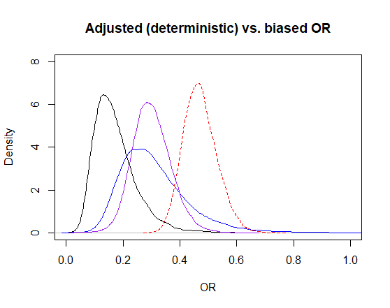
Figure. OR biased (red dashed) and adjusted posterior distributions estimated using a stochastic approach (purple = exposure misclassification-adjusted, blue = selection bias + exposure misclassification-adjusted, black = confounding + selection bias + exposure misclassification-adjusted.