Chapitre 7 Selection bias
Selection bias will arise when a measured of association between an exposure and a disease is wrongly conditioned on a third variable. For instance, if we were to control the S variable in the figure below.

Figure. DAG representation of selection bias by a variable S.
Remember, we can condition on a variable:
1. by selecting study subjects that all have the same value for the variable (exclusion);
2. by matching subjects based on this value (matching);
3. by including the variable in our model in multiple regression (analytical control).
In the DAG above, we see that conditioning on S is opening a path that was otherwise closed (S collides between exposure-disease).
Of course, if the selection bias was introduced by analytical control, well… Just remove the unneeded variable from your model! Otherwise, to adjust for a selection bias due to the study design, we can use a conventional logistic model in a Bayesian framework, within which the adjustment for selection bias described by Lash et al. (2009) is incorporated within the estimation process.
With:
- \(S(d+e+)\) being the probability of being selected if diseased and exposed;
- \(S(d+e-)\) being the probability of being selected if diseased and unexposed;
- \(S(d-e-)\) being the probability of being selected if healthy and unexposed;
- \(S(d-e+)\) being the probability of being selected if healthy and exposed;
We can compute what is called the selection OR (\(OR(sel)\)) as follows:
\(OR(sel) = \frac{S(d+e-)*S(d-e+)}{S(d+e+)*S(d-e-)}\)
Then, we can compute an adjusted OR (\(OR(adj)\)) simply by multiplying the biased OR (\(OR(biased)\)) by the \(OR(sel)\). This \(OR(adj)\) now describe the relation between exposure and disease after adjusting for the selection bias.
\(OR(adj) = OR(biased) * OR(sel)\)
or
\(OR(adj) = OR(biased) * \frac{S(d+e-)*S(d-e+)}{S(d+e+)*S(d-e-)}\)
We could thus, simply:
1. Provides prior distributions for the intercept, the coefficient of interest, but also for the 4 selection bias parameters (\(S(d+e-)\), \(S(d-e+)\), \(S(d+e+)\), and \(S(d-e-)\)).
NOTE THAT: instead of providing prior distributions for the bias parameters, you could also specify an exact value for these (e.g., \(S(d+e-)=0.15\)). The adjustment would then be deterministic, rather than stochastic, for the biased parameters;
2. Develop a conventional logistic Bayesian model;
3. Include the above equation to compute the \(OR(adj)\).
If we use uniform vague distributions for the intercept and the coefficient of interest:
options(scipen=999) # To avoid use of scientific notation by R

mu_int <- 0.0         #mu for the intercept
inv_var_int <- 0.0001 #Inverse variance for the intercept
mu_betaquest <- 0.0   #mu for the coefficient
inv_var_betaquest <- 0.0001 #Inverse variance for the coefficient
We could use beta distributions for the selection bias parameters, since these are all probabilities (i.e., we would like to bound them between 0.0 and 1.0). Here, we will need to use the epi.betabuster() function from the epiR library to identify the a and b shape parameters for each distribution.
For instance, if we believe that:
- \(S(d+e+)\) has mode of 0.75 and that we are 95% certain that it is above 0.65;
- \(S(d+e-)\) has mode of 0.25 and that we are 95% certain that it is below 0.35;
- \(S(d-e+)\) has mode of 0.30 and that we are 95% certain that it is below 0.40;
- \(S(d-e-)\) has mode of 0.10 and that we are 95% certain that it is below 0.20;
We could find the 4 corresponding beta distributions as follow:
library(epiR)
#S(Dis+ Exp+)
rval.dis.exp <- epi.betabuster(mode=0.75, conf=0.95, greaterthan=T, x=0.65)
rval.dis.exp$shape1
## [1] 48.603rval.dis.exp$shape2 ## [1] 16.86767#plot the prior distribution
curve(dbeta(x, shape1=rval.dis.exp$shape1, shape2=rval.dis.exp$shape2), from=0, to=1,
main="Prior for S(d+e+)", xlab = "Proportion", ylab = "Density")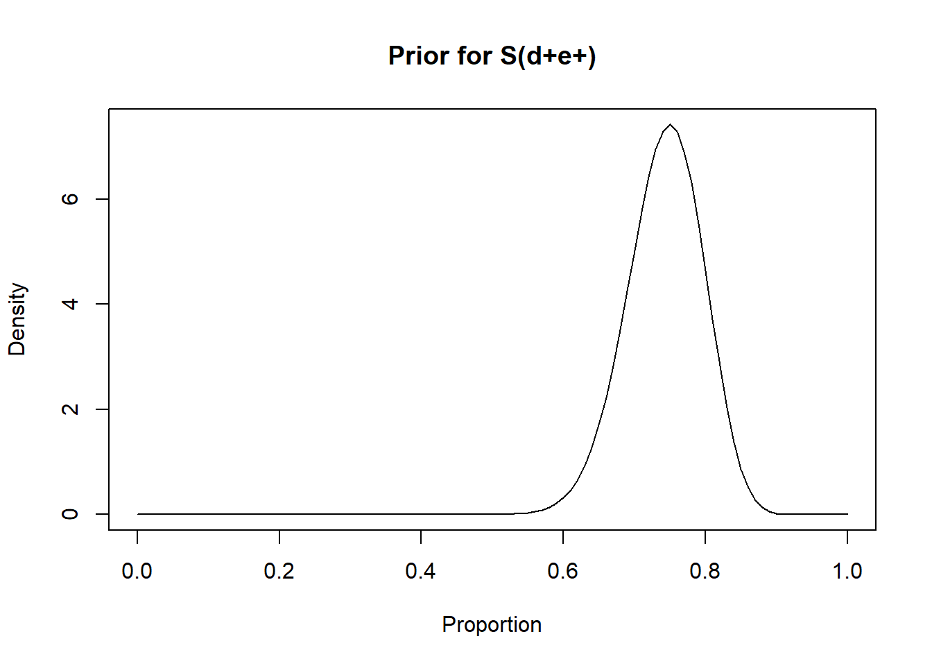
#S(Dis+ Exp-)
rval.dis.unexp <- epi.betabuster(mode=0.25, conf=0.95, greaterthan=F, x=0.35)
rval.dis.unexp$shape1
## [1] 16.868rval.dis.unexp$shape2 ## [1] 48.604#plot the prior distribution
curve(dbeta(x, shape1=rval.dis.unexp$shape1, shape2=rval.dis.unexp$shape2), from=0, to=1,
main="Prior for S(d+e-)", xlab = "Proportion", ylab = "Density")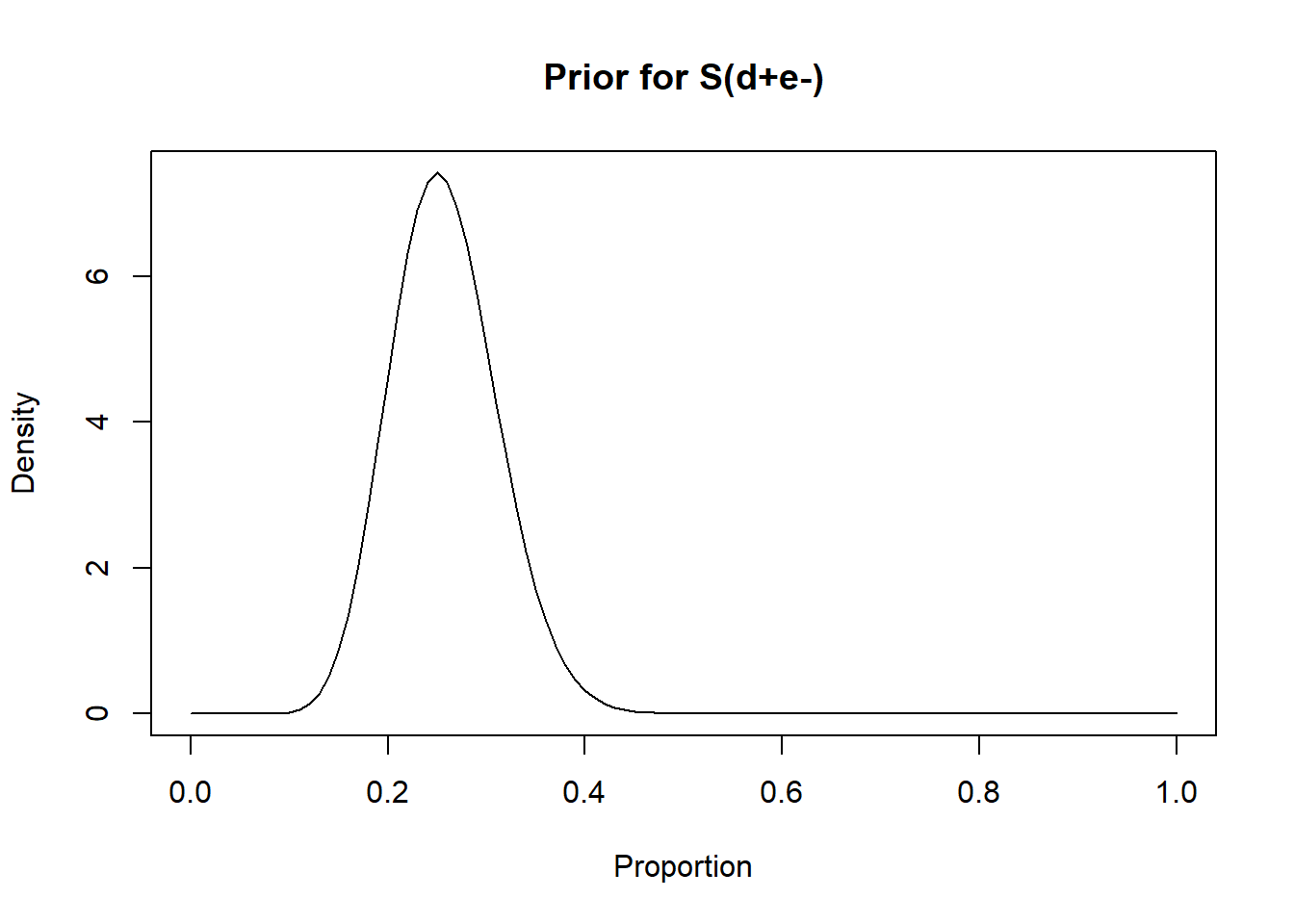
#S(Dis- Exp+)
rval.undis.exp <- epi.betabuster(mode=0.30, conf=0.95, greaterthan=F, x=0.40)
rval.undis.exp$shape1
## [1] 20.939rval.undis.exp$shape2 ## [1] 47.52433#plot the prior distribution
curve(dbeta(x, shape1=rval.undis.exp$shape1, shape2=rval.undis.exp$shape2), from=0, to=1,
main="Prior for S(d-e+)", xlab = "Proportion", ylab = "Density")
#S(Dis- Exp-)
rval.undis.unexp <- epi.betabuster(mode=0.10, conf=0.95, greaterthan=F, x=0.20)
rval.undis.unexp$shape1
## [1] 5.619rval.undis.unexp$shape2 ## [1] 42.571#plot the prior distribution
curve(dbeta(x, shape1=rval.undis.unexp$shape1, shape2=rval.undis.unexp$shape2), from=0, to=1,
main="Prior for S(d-e-)", xlab = "Proportion", ylab = "Density")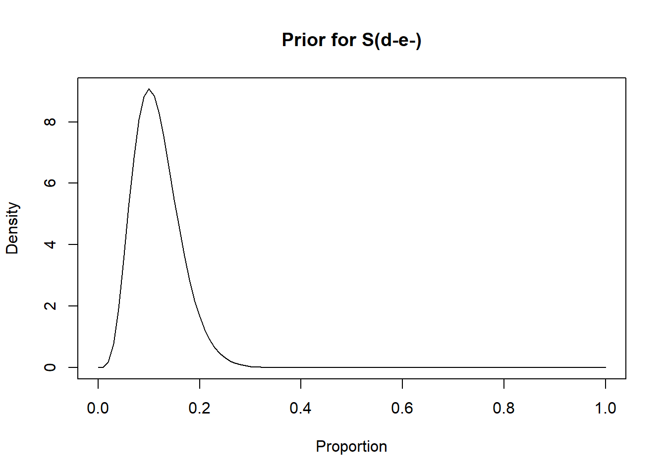
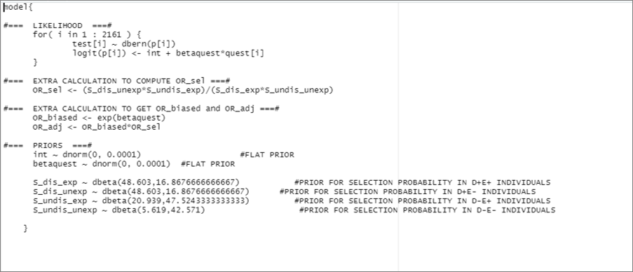
With these priors being determined, the following code would create the text file for the model:
# Specify the model:
model_sel <- paste0("model{

#===    LIKELIHOOD  ===#
            for( i in 1 : ",num_obs," ) {
                            test[i] ~ dbern(p[i])
                            logit(p[i]) <- int + betaquest*quest[i]
            }

#===  EXTRA CALCULATION TO COMPUTE OR_sel ===#
            OR_sel <- (S_dis_unexp*S_undis_exp)/(S_dis_exp*S_undis_unexp)

#===  EXTRA CALCULATION TO GET OR_biased and OR_adj ===#
            OR_biased <- exp(betaquest)
            OR_adj <- OR_biased*OR_sel

#===    PRIORS  ===#
            int ~ dnorm(",mu_int,", ",inv_var_int,")                        #FLAT PRIOR
            betaquest ~ dnorm(",mu_betaquest,", ",inv_var_betaquest,")  #FLAT PRIOR

            S_dis_exp ~ dbeta(", rval.dis.exp$shape1,",",rval.dis.exp$shape2, ")               #PRIOR FOR SELECTION PROBABILITY IN D+E+ INDIVIDUALS
            S_dis_unexp ~ dbeta(", rval.dis.unexp$shape1,",",  rval.dis.unexp$shape2, ")          #PRIOR FOR SELECTION PROBABILITY IN D+E- INDIVIDUALS
            S_undis_exp ~ dbeta(",  rval.undis.exp$shape1,",", rval.undis.exp$shape2, ")             #PRIOR FOR SELECTION PROBABILITY IN D-E+ INDIVIDUALS
            S_undis_unexp ~ dbeta(", rval.undis.unexp$shape1,",", rval.undis.unexp$shape2, ")                       #PRIOR FOR SELECTION PROBABILITY IN D-E- INDIVIDUALS

        }")

#write to temporary text file
write.table(model_sel, file="model_sel.txt", quote=FALSE, sep="", row.names=FALSE,
 col.names=FALSE)
This code would create the following .txt file:
Again, if we want to provide initial values, we will have to provide them for all the unknown parameters (including the selection probabilities). So, not just int and betaquest, but also \(S(d+e-)\), \(S(d-e+)\), \(S(d+e+)\), and \(S(d-e-)\). For instance:
inits <- list(
  list(int=0.0, betaquest=0.0, S_dis_exp=0.20, S_dis_unexp=0.20, S_undis_exp=0.20, S_undis_unexp=0.20),
  list(int=1.0, betaquest=1.0, S_dis_exp=0.30, S_dis_unexp=0.30, S_undis_exp=0.30, S_undis_unexp=0.30),
  list(int=-1.0, betaquest=-1.0, S_dis_exp=0.40, S_dis_unexp=0.40, S_undis_exp=0.40, S_undis_unexp=0.40)
)
When you will run the Bayesian analysis, again you will have to modify the parameters that you want to monitor:
library(R2OpenBUGS)
#Set number of iterations
niterations <- 5000
#Run the Bayesian model
bug.out.sel <- bugs(data=cyst,
                inits=inits,
                parameters.to.save=c("int", "betaquest", "OR_sel", "OR_biased", "OR_adj"),    ### HERE I HAVE ADDED OR_sel, OR_biased, and OR_adj ###
                n.iter=niterations,
                n.burnin=0,
                n.thin=1,
                n.chains=3,
                model.file="model_sel.txt",
                debug=FALSE,
                DIC=FALSE)