Chapitre 3 Running a logistic model
OpenBUGS is one of the most used Bayesian software. It is a bit tedious to use, though, and it requires a lot of “point and click,” which reduce reproducibility. Although OpenBUGS can be used with a script mode (i.e., coding vs. point and click), it is a lot easier to operate OpenBUGS within R. The R2OpenBUGS library provides a R interface that will use OpenBUGS for conducting Bayesian analyses. The codes that you have used in R can easily be saved and re-used or modified later. The output generated through R can later be used to produce figures or results tables for publication.
Basically, to run a given model in OpenBUGS we will need:
- Data
- A model containing:
- A likelihood function linking observed data to unknown parameters
- A prior distribution for each unknown parameter
- An initial value for each unknown parameters to start the Markov chains
- These values can also be generated randomly by the software, but specifying them will improve reproducibility
3.1 The data
This is the easy part. For these exercises we provided the datasets as CSV files. The function read.csv() can be used to upload a CSV dataset. In the R projects that you will use for the exercises, we always stored the datasets in a folder named Data. For the exercises, we will use the study dataset (cyst_bias_study.csv).
Below we imported the dataset, named it cyst, and checked the first 6 rows using the head() function.
#Upload the .csv dataset:
cyst <- read.csv(file="Data/cyst_bias_study.csv", header=TRUE, sep=";")
head(cyst)
## id cyst test know quest sw lat rand
## 1 2 NA 0 NA 1 1 0 1
## 2 5 NA 0 NA 1 0 1 0
## 3 9 NA 0 NA 1 1 1 1
## 4 10 NA 1 NA 1 0 0 1
## 5 13 NA 1 NA 0 1 0 0
## 6 15 NA 0 NA 1 1 0 1We will focus for now on the variable test as our outcome (i.e., whether or not the individual was positive for cysticercosis; this is a version of cyst with some misclassification included). We will use quest as our main predictor (whether or not the individual scored “knowledgeable for cysticercosis”; this is a version of know with some misclassification included).
We can check how many rows (i.e., how many observations) the dataset contains using the dim() function. This function create a small list with two values, the first one is the number of row, the second one is the number of columns. In the code below, I am saving that number of observations (named num_obs) for later usage.
#Create a "a" object with number of rows and columns
  a <- dim(cyst)
#Save and check the first value of the "a" object
  num_obs <- a[1]
  num_obs
## [1] 2161There are 2161 observations in the dataset.
3.2 The model
3.2.1 The likelihood function
For a conventional logistic regression we could describe the likelihood function linking unknown parameters to observed data as follow:
\(test \sim dbern(P)\)
\(logit(P) = β_0 + β_1*quest\)
In other words: the outcome test follows a Bernoulli distribution (i.e., it can take the value 0 or 1) with probability P of the value being a 1. The logit of this probability is described by an intercept (\(β_0\)) and a coefficient (\(β_1\)). The latter is multiplied by the value of the predictor quest.
In this case, the values of test and quest are the observed data and the intercept (\(β_0\)) and coefficient (\(β_1\)) are the unknown parameters.
3.2.2 Priors for unkown parameters
We will have to specify a prior distribution for each unknown parameter (using the \(\sim\) sign) or to assign a specific value to it (using the \(<-\) sign). With the former, we allow for a range of values (stochastic), while the latter would be a deterministic approach.
In the preceding example, we only have an intercept (\(β_0\)) and a coefficient (\(β_1\)). Theoretically such parameters could take values from -infinite to +infinite, so a normal distribution would be one way to describe their prior distributions. Moreover, if we want to use flat priors, we could simply choose \(mu=0.0\) and \(1/tau=0.0001\) to describe these distributions (i.e., centred on 0.0 with a large variance; \(var = 10,000\)).
In the following code, I am creating R objects for mu and 1/tau (i.e., the inverse of the variance) for \(β_0\) and for \(β_1\) prior distributions.
options(scipen=999) # To avoid use of scientific notation by R

mu_int <- 0.0         #mu for the intercept
inv_var_int <- 0.0001 #Inverse variance for the intercept
mu_betaquest <- 0.0   #mu for the coefficient
inv_var_betaquest <- 0.0001 #Inverse variance for the coefficient
3.2.3 Creating the OpenBUGS model
Our Bayesian model has to be presented to OpenBUGS as a text file (i.e., a .txt document). To create this text file, we will use the paste0() function to write down the model and then the write.table() function to save it as a .txt file.
An interesting feature of the paste0() function is the possibility to include R objects in the text. For instance, you may want to have a general model that will not be modified, but to change the values used to describe the priors. Within your paste0() function you could call these “external” values. Thus, you just have to change the value of the R object that your model is using, rather than rewriting a new model. For instance, we already created a R object called num_obs (which is just the number of observations in the dataset). We can create a short text as follow:
text1 <- paste0("for( i in 1 : 2161 )")
text1
## [1] "for( i in 1 : 2161 )"But, if the model is to be applied later to another dataset with a different number of observations, it may be more convenient to use:
text2 <- paste0("for( i in 1 : ",num_obs," )")
text2
## [1] "for( i in 1 : 2161 )"When using paste0(), any text appearing between sets of quotations marks and within commas (i.e.," “,bla-bla,” ") will be considered as a R object that need to be included between the pieces of text included in each quotation.
Some important notes:
OpenBUGS is expecting to see the word “model” followed by curly brackets { }. The curly brackets will contain the likelihood function AND the priors.
Similarly to
R, any line starting with a # will be ignored (these are comments).Similarly to
R, <- means equal.The ~ symbol means “follow a distribution.”
Similarly to
ROpenBUGS is case sensitive (i.e., ORQUEST does not equal orquest).Loops can be used with keyword “for” followed by curly brackets.
Array can be indicated using squared brackets [ ].
In the example below, I create a R object called model using the paste0() function and then save it as a text file using the write.table() function. We will check this text file below and then explain the code for the model.
# Specify the model:
model <- paste0("model{

#===    LIKELIHOOD  ===#
            for( i in 1 : ",num_obs," ) {
                            test[i] ~ dbern(p[i])
                            logit(p[i]) <- int + betaquest*quest[i]
            }

#===   EXTRA CALCULATION TO GET OR ===#
            ORquest <- exp(betaquest)

#===    PRIOR   ===#
            int ~ dnorm(",mu_int,", ",inv_var_int,")        #FLAT PRIOR
            betaquest ~ dnorm(",mu_betaquest,", ",inv_var_betaquest,")  #FLAT PRIOR
            }")

#write to temporary text file
write.table(model, file="model.txt", quote=FALSE, sep="", row.names=FALSE,
 col.names=FALSE)
Here is a snapshot of the final result (i.e., the text file):
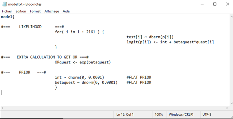
If we look more closely at the likelihood function:
for( i in 1 : 2161 ) {
test[i] \(\sim\) dbern(p[i])
logit(p[i]) <- int + betaquest*quest[i]
}
It is read by OpenBUGS as:
- For observation #1, the observed value for test (test[1]) follows a Bernoulli distribution with a probability (p[1]) that it is equal to 1. This probability is linked to a combination of linear predictors, through the logit function, and is function of the observed quest value (quest[1]).
- For observation #2, the observed value for…
- …
- For observation #2161, the observed value for…
So, on a given iteration, the software will go through the entire dataset to try to assess the potential values for our unknown parameters (int and betaquest).
In the next piece of code:
ORquest <- exp(betaquest)
We are just transforming the coefficient for the variable quest into an \(OR\) using the exponent of betaquest.
The last part is simply the specification of our prior distributions for the two unknown parameters (int and betaquest).
3.3 Generating initial values
The initial value is the first value where each Markov chain will start.
- You can specify one value for each parameter for which you have
specified a distribution (~) in the model.
- If you decide to ran three Markov chains, you will need three
different sets of initial values.
For instance, in our preceding example we have two unknown parameters (int and betaquest). If we were to run three Markov chains, we could generate three sets of initial values for these two parameters as follow. Of course, the chosen values could be changed.
#Initializing values for 3 chains
inits <- list(
  list(int=0.0, betaquest=0.0),
  list(int=1.0, betaquest=1.0),
  list(int=-1.0, betaquest=-1.0)
  )
We know have a R object that I have called inits and it contains the values where each of the three Markov chains will start.
3.4 Running model in OpenBUGS
We now have the three elements that we needed: data, a model, and a set of initial values. We can now use the R2OpenBUGS library to run our Bayesian analysis. The function that we will use for that is the bugs() function. Here are the arguments that we need to specify:
- The dataset using
data=
- The sets of initial values using
inits=
- The names of the parameters which should be monitored using
parameters.to.save=
- The number of total iterations per chain (including burn in; default: 2000) using
n.iter= - The length of burn in (i.e., number of iterations to discard at the beginning) using
n.burnin=. - The thinning rate using
n.thin=. Must be a positive integer. The default is n.thin = 1 (no thinning).
- The number of Markov chains using
n.chains=. The default is 3.
- The text file containing the model written in OpenBUGS code using
model.file=.
The debug=TRUE or debug=FALSE argument is controlling whether OpenBUGS remains open after the analysis. If FALSE (default), OpenBUGS is closed automatically when the script has finished running, otherwise OpenBUGS remains open for further investigation. Keeping the software open will help investigating any error message. However, R will then wait for you to close OpenBUGS before continuing with any subsequent lines of code. In situations where many analyses are ran sequentially, then it may be advantageous to have the software to close automatically after each analysis.
The last argument DIC=TRUE or DIC=FALSE will determine whether to compute the deviance, pD, and deviance information criteria (DIC). These could sometimes be useful for model selection/comparison. We could leave that to DIC=FALSE since we will not be using these values in the workshop.
When conducting any analysis, OpenBUGS will go through these steps and will provide these associated messages (if everything is fine):
– Making sure the model in the text file is sound. Message: Model is syntactically correct
– Loading the data. Message: Data loaded
– Making sure that the model and data correspond. Message: Model compiled
– Loading the initial values. Message: Initial values loaded
– Making sure that all unknown parameters have initial values (and generating them if you have not fully specified them). Message: Model is initialized
- Starting the update (i.e., running the Markov chains as specified). Message: Model is updating
Do not worry if you appear to be stuck on this last step. Bayesian analyses are an iterative process, with a moderate size dataset, it may take a few seconds or minutes to complete the process. On my computer, the following model took 38 seconds to run.
With the following code, we will create a R object called bug.out. This object will contains the results of running our model, with the specified priors, using the available data, and the sets of initial values that we have created. For this analysis, we have asked to run 3 Markov chains, each for 5000 iterations and we discarded 0 iteration (so we have not yet specified a proper burn in period). Finally, we will monitor our two main unknown parameters (int and betaquest) and the computed \(OR\) for quest (ORquest).
library(R2OpenBUGS)
#Set number of iterations
niterations <- 5000

#Run the Bayesian model
bug.out <- bugs(data=cyst,
                inits=inits,
                parameters.to.save=c("int", "betaquest", "ORquest"),
                n.iter=niterations,
                n.burnin=0,
                n.thin=1,
                n.chains=3,
                model.file="model.txt",
                debug=FALSE,
                DIC=FALSE)
3.5 Model diagnostic
Before jumping to the results, you should first check:
- Whether the chains have converged,
- What the burn in period should be or, if you already specified one, if it was sufficient,
- Whether you have a large enough sample of values to describe the posterior distribution with sufficient precision,
- Whether the Markov chains behaved well (mainly their auto-correlation).
There are many other diagnostic methods available for Bayesian analyses, but, for this workshop, we will mainly use basic methods relying on plots.
Diagnostics are available when you convert your model output into an MCMC object using the as.mcmc() function of the mcmcplot library.
library(mcmcplots)
bug.mcmc <- as.mcmc(bug.out)
You can then use the mcmcplot() function on this newly created MCMC object.
mcmcplot(bug.mcmc, title="Diagnostic plots")When you do that, a HTML document will be created an your web browser will automatically open it. Here is a snapshot of the HTML file in my browser:
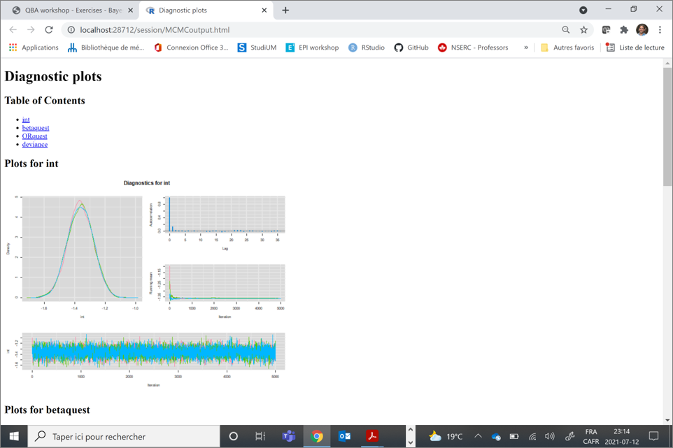
3.5.1 Convergence and burn-in
To check whether convergence of the Markov chains was obtained you can inspect the trace plot presenting the values that were picked by each chain on each iterations. The different chains that you used (three in the preceding example) will be overlaid on the trace plot. You should inspect the trace plot to evaluate whether the different chains all converged in the same area. If so, after a number of iterations they should be moving in a relatively restricted area and this area should be the same for all chains.
Here is an example of a trace plot of three “nice” Markov chains (from our preceding example, lucky us!).
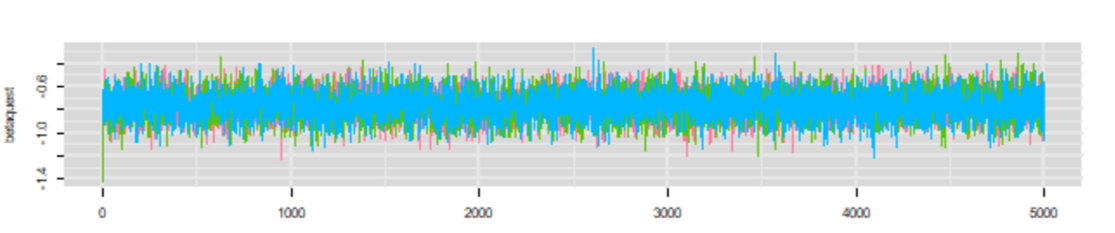
In this preceding example, we can see that the chains started from different initial values, but they very quickly converged (after less than a 100 iterations) toward the same area. They were then moving freely within this limited area (thus sampling from the posterior distribution). We could conclude based on this trace plot that:
- The Markov chains did converged
- A short burn in period of less than a 100 iterations would be sufficient. Note that we will often use longer burn in (e.g., 1000) just to be sure and because it only costs a few more seconds on your computer…
Here is another example where two chains (the red and green) converged in the same area, but a third one (the blue) also converged, but in a different area. We should be worry in such case.
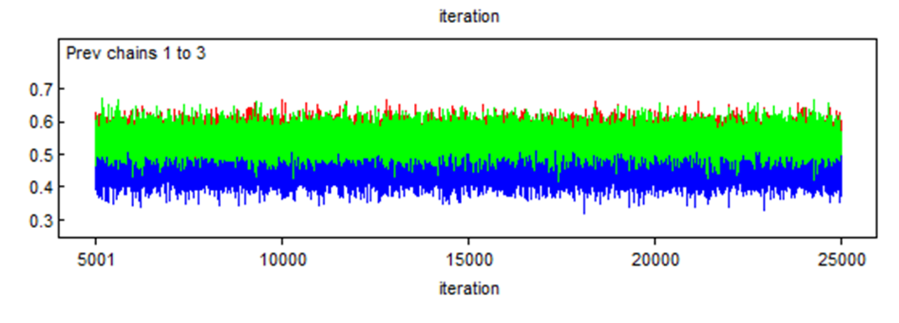
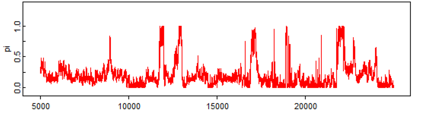
Finally, here is a last example with just one Markov chain and it clearly did not converged, even after 25,000 iterations. You should be terrified by that!!! ;-).
3.5.2 Number of iterations
Next, you can inspect the posterior distributions to determine if you have a large enough sample of independent values to describe with precision the median estimate and the 2.5th and 97.5th percentiles. The effective sample size (EES) takes into account the number of values generated by the Markov chains AND whether these values were autocorrelated, to compute the number of “effective” independent values that are used to described the posterior distribution. Chains that are autocorrelated will generate a smaller number of “effective values” than chains that are not autocorrelated.
The effectiveSize() function of the coda library provide a way to appraise whether you add enough iterations. In the current example, we already created a mcmc object named bug.mcmc. We can ask for the effective sample size as follow:
effectiveSize(bug.mcmc)## int betaquest ORquest
## 11009.48 10433.54 10675.81You could, for example, decide on an arbitrary rule for ESS (say 10,000 values) and then adapt the length of the chain to achieve such an ESS (for each of the selected parameters, because the effective sample sizes will not be the same for all parameters).
3.5.3 Autocorrelation
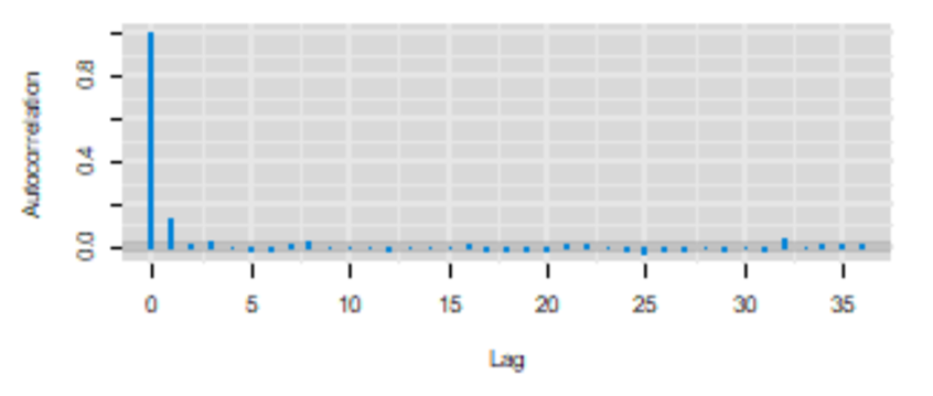
Remember, a feature of Markov chains is to have some autocorrelation between two immediately subsequent iterations and then a correlation that quickly goes down to zero (i.e., they have a short memory). The autocorrelation plot can be used to assess if this feature is respected.
From our previous example, it seems that it is the case.
Here is another example that should be worrying.
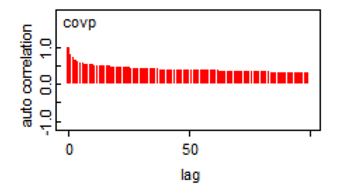
When such a behaviour is observed, running the chains for more iterations will achieve the desire ESS. In some situations, specifying different priors (i.e., increasing the amount of information in priors) may also help.
3.6 Getting our estimates
Now, if you are happy with the behaviour of your Markov chains and you determined what would be an appropriate number of iterations and burn in period, you are left with two options:
- You could go back and run again the
R2OpenBUGSbugs()function, while adjusting the burn in (n.burnin=) and, if needed, the number of iterations (n.iter=). For publication, THIS IS THE ABSOLUTE BEST OPTION, because you will then have the exact ESS, trace plots, etc.
- However, if these are preliminary analyses and your number of iterations was already sufficient, you could simply use the output that you already have and remove retrospectively the values sampled by the Markov chains during the burn in period. It will save you from running
R2OpenBUGSagain.
3.6.1 Re-run R2OpenBUGS
For a final analysis (e.g., for publication), you will re-run the bugs() function, and indicate a burn in period (e.g., n.burnin=1000). If needed, you could also increase the number of iterations (n.iter=) if the ESS was too small. For instance, in the code below, I kept the number of iteration unchanged (n=5,000), but indicated a burn in period of 1,000 iterations :
library(R2OpenBUGS)
#Set number of iterations
niterations <- 5000
nburnin <- 1000
#Run the Bayesian model
bug.out <- bugs(data=cyst,
                inits=inits,
                parameters.to.save=c("int", "betaquest", "ORquest"),
                n.iter=niterations,
                n.burnin=nburnin,
                n.thin=1,
                n.chains=3,
                model.file="model.txt",
                debug=FALSE,
                DIC=FALSE)
When you have specified the burn in period directly in the bugs() function, you can summarize your results (i.e., report the median, 2.5th and 97.5th percentiles) very easily with the print() function. Below, I have also indicated digits.summary=3 to adjust the precision of the estimates that are reported (the default is 1).
print(bug.out, digits.summary=3)## Inference for Bugs model at "model.txt",
## Current: 3 chains, each with 5000 iterations (first 1000 discarded)
## Cumulative: n.sims = 12000 iterations saved
## mean sd 2.5% 25% 50% 75% 97.5% Rhat n.eff
## int -1.363 0.084 -1.527 -1.420 -1.362 -1.306 -1.201 1.001 12000
## betaquest -0.761 0.124 -1.005 -0.845 -0.761 -0.677 -0.519 1.001 12000
## ORquest 0.471 0.058 0.366 0.430 0.467 0.508 0.595 1.001 12000
##
## For each parameter, n.eff is a crude measure of effective sample size,
## and Rhat is the potential scale reduction factor (at convergence, Rhat=1).Here you see that the median OR estimate (95CI) was 0.47 (0.37, 0.60).
Finally, we could also plot the prior and posterior distributions on a same figure (rather than just reporting the median and 95 credible interval). Below, I will create a plot with the prior and posterior distributions for the estimated coefficient of the quest variable.
First, if you inspect the bug.out object that was created using R2OpenBUGS, you will notice a sims.list object which is made of 3 lists (one for each of the 3 parameters that were monitored; int, betaquest, and ORquest). Each list is made of 12,000 values, which are the values from the three chains assembled together (5000 values minus a burn in of 1000, and, finally, times 3 chains).
For plotting these values, I can use the plot() function. More specifically, I asked for a density curve (density()) of my estimate (in our case, the betaquest list in the sims.list element of the bug.out object. Using $ signs indicate the variable, in the list, of the object.
Then, I could add to this plot my prior distribution for that same parameter. Remember, for OpenBUGS, I have specified that this parameter followed a Normal distribution with mean=mu_betaquest (0.0) and inverse variance=inv_var_betaquest (0.0001). The curve() function, however, requires the mean and standard deviation (SD) to plot a given Normal distribution. Therefore, I first computed this standard deviation (which is the square root of the variance, or , in this case, the square root of the inverse of the inverse variance) and then asked for a Normal curve with this mean and SD.
The lty= option indicate the line type (2 is for dashed) and the add=TRUE argument simply indicates to put both curves on the same plot.
#Computing the SD for my prior distribution
std <- sqrt(1/inv_var_betaquest)

#Plotting the posterior distribution
plot(density(x=bug.out$sims.list$betaquest),
     main="Quest coefficient",
     xlab="Value", ylab="Density",
     )
#Adding the prior distribution
curve(dnorm(x,
            mean=(mu_betaquest),
            sd=std
            ),
      lty=2,
      col="red",
      add=TRUE
      )
Figure 3.1: Figure. Prior (dashed red line) and posterior (full black line) distribution of the coefficient for the variable quest.
In this example, since the prior distribution was a vague distribution, the prior distribution is not obvious on the figure, it is the straight dashed red line at the bottom of the figure.
3.6.2 Using already available output
Throughout the exercises, I will use this option most of the time, but remember this is just for preliminary analyses. When you are ready for publication, run the R2OpenBUGS script with the appropriate number of iterations and burn in period.
Nonetheless, if we want to use the already available output, you could use the seq() function which is a basic R function to specify the first iteration to keep (using from=) and the last iteration to keep (using to=). The by=1 argument, indicates that each values are to be retained. For instance, by=2, would indicate to keep every other value. As an example, with the code below, I am creating a R object named k which is simply a list of values from 1001 to 5000 by increment of 1. I will later combine this list with my bug.out object to identify the values from my Markov chains that are to be kept.
# Set burn-in to 1000
burnin <- 1000
# Create a sequence of values between 1001 and 5001
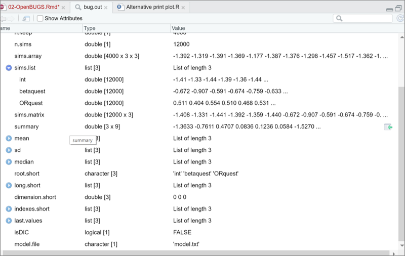
k <- seq(from=(burnin+1), to=niterations, by=1)Now, if you inspect the bug.out object that was created earlier using R2OpenBUGS, you will notice an element named sims.array. As you can see below, this element is made of 3 times 3 lists of 5000 values. This correspond to the 5000 values sampled (1/iteration) by each Markov chain (3 chains) for the 3 parameters that were monitored (int, betaquest, and ORquest). Within this element, the chains were not assembled together yet.
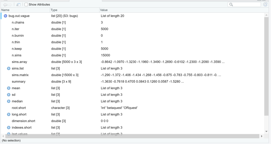
Figure. sims.array element of the bug.out R2OpenBUGS output.
We could combine these values using the data.frame() and rbind() functions with the list of iteration k that I created to organize a dataset where I have all the values from the three Markov chains for a given parameter in a same column, and where the values belonging to the burn in period are now excluded, retrospectively.
# Combine chains post-burn in
estimates_conv_logistic <- data.frame(rbind(bug.out$sims.array[k,1,],bug.out$sims.array[k,2,],bug.out$sims.array[k,3,]))
dim(estimates_conv_logistic)
## [1] 12000 3Here we can see that it is a dataset with 12,000 rows (3 Markov chains times 4000 iterations [5000 iterations minus the burn in of 1000 iterations]) and 3 columns. Below are the first 6 observations from this dataset.
head(estimates_conv_logistic)## int betaquest ORquest
## 1 -1.392 -0.8091 0.4453
## 2 -1.319 -0.7896 0.4540
## 3 -1.391 -0.7062 0.4935
## 4 -1.369 -0.7952 0.4515
## 5 -1.177 -0.8776 0.4158
## 6 -1.387 -0.7423 0.4760All that we have left to do now, is to compute the median and 2.5th and 97.5th percentiles for the parameters of interest. For that, we can use the apply() function. We need to indicate:
- the dataset to use (X=),
- whether it is the rows (MARGIN=1), or columns (MARGIN=2) for which descriptive statistics must be computed (in this case we wish to obtain descriptive statistic for each column),
- the actual descriptive statistic that we need (FUN=; in this case we want the quantiles, FUN=quantile),
- and, finally, arguments that are specific to the chosen descriptive statistic; here the percentiles that we would like to have reported (probs=c(0.5, 0.025, 0.975)).
# medians and 95% credible intervals
a <- apply(X=estimates_conv_logistic, MARGIN=2, FUN=quantile, probs=c(0.5, 0.025, 0.975))
a
## int betaquest ORquest
## 50% -1.362 -0.761150 0.4671000
## 2.5% -1.527 -1.005025 0.3659000
## 97.5% -1.201 -0.518895 0.5952025Since it is not super nice to have the parameters as columns and statistic as rows, we could transpose this table using the t() function.
b <- t(a)
b
## 50% 2.5% 97.5%
## int -1.36200 -1.527000 -1.2010000
## betaquest -0.76115 -1.005025 -0.5188950
## ORquest 0.46710 0.365900 0.5952025Finally, rounding off a bit never hurts. The round() function can be used for that.
res_conv_logistic <- round(b, digits=3)
res_conv_logistic
## 50% 2.5% 97.5%
## int -1.362 -1.527 -1.201
## betaquest -0.761 -1.005 -0.519
## ORquest 0.467 0.366 0.595Of course, all of this can be done in one single step.
res_conv_logistic <- round(
  t(
    apply(X=estimates_conv_logistic, MARGIN=2, FUN=quantile, probs=c(0.5, 0.025, 0.975))
    ),
  digits=3)
Finally, we could also plot the prior and posterior distributions on a same figure, but we would now use the variable betaquest in the data frame estimates_conv_logistic, or estimates_conv_logistic$betaquest).
std <- sqrt(1/inv_var_betaquest)

plot(density(x=estimates_conv_logistic$betaquest),
     main="Quest coefficient",
     xlab="Value", ylab="Density",
     )
curve(dnorm(x,
            mean=(mu_betaquest),
            sd=std
            ),
      lty=2,
      col="red",
      add=TRUE
      )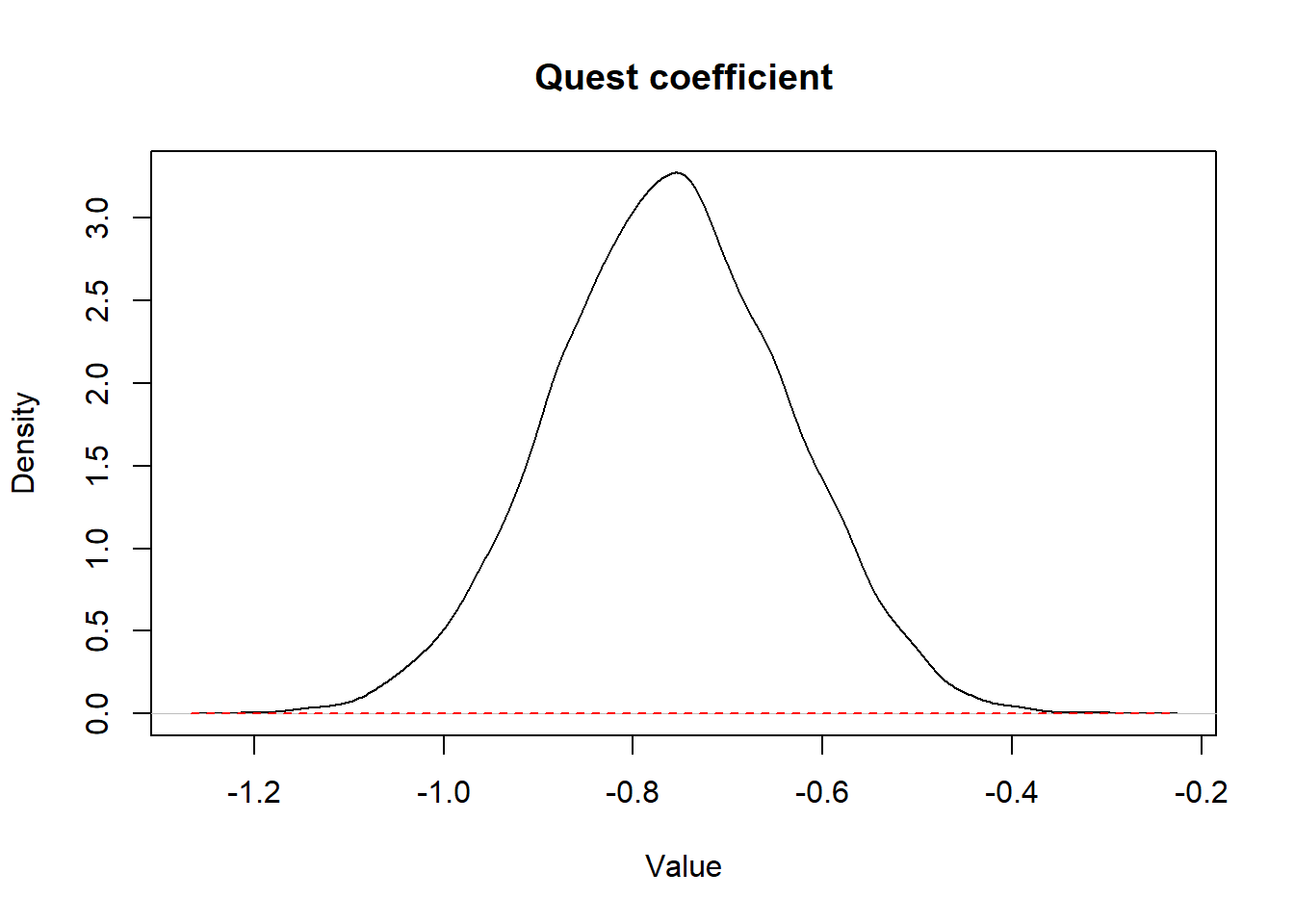
Figure 3.2: Figure. Prior (dashed red line) and posterior (full black line) distribution of the coefficient for the variable quest.